Realtime Monocular Depth Mapping
Real-time monocular depth mapping using lightweight U-Net architecture.

A PyTorch-based depth mapping project using the NYU dataset. This implementation includes various neural network architectures for single image depth prediction with custom loss functions and data augmentation.
Realtime Single Image Depth Mapping
Short Description
A U-Net based convolutional neural network for estimating depth from a single RGB image, designed to run at real-time inference speed. The model surpasses a standard U-Net baseline in accuracy while being significantly smaller and faster, making it suitable for applications like self-driving technology, robotics, and medical surgery.
Overview
This project focuses on monocular depth mapping from single RGB images using deep neural networks. Depth mapping is a critical task in computer vision with applications in robotics, autonomous driving, 3D reconstruction, and scene understanding. This work implements and compares multiple network architectures (Autoencoder and UNet) trained on the NYU Depth dataset. Our approach combines multiple loss functions including SSIM loss and gradient-based depth loss to improve depth prediction quality. The implemented methods achieve competitive accuracy with efficient computational performance suitable for real-time applications.

Problem Statement
Single image depth mapping is an ill-posed problem due to structural and material ambiguities (e.g., reflective surfaces). Unlike stereo depth mapping, no second viewpoint is available to resolve correspondence, so the network must infer depth using cues such as line angles, perspective, object size, parallelism, and semantic features. The goal of this project was to design a network that:
- Predicts accurate dense depth maps from a single RGB image
- Runs at real-time inference speed (targeting \(\sim 24–30\) FPS)
- Improves on existing baseline approaches in both accuracy and efficiency
Solution
The project formulates single image depth mapping as a supervised regression task, where a CNN N maps an RGB image I_c to a predicted depth image I_d:
I_d = N(I_c)
A U-Net-based encoder-decoder architecture was designed and trained using a combined loss function targeting low-frequency similarity, perceptual/structural similarity, and high-frequency edge accuracy. The model was benchmarked against the original U-Net architecture (proposed for biomedical image segmentation) as a baseline.
Key Features
- Custom lightweight U-Net-based encoder-decoder architecture for depth regression
- Bilinear upsampling in the decoder to avoid checkerboard artifacts common with transpose convolutions
- Skip connections between encoder and decoder blocks to preserve high-frequency detail (e.g., edges) lost during max pooling
- Combined loss function integrating three complementary objectives (L1, Structural, and Depth Gradient losses)
- \(\sim 14 \times\) fewer parameters than the baseline U-Net
- \(\sim 6 \times\) faster inference than the baseline, achieving 35.5 FPS
- Data augmentation via random horizontal flip and random rotation (up to \(15^\circ\))
Research Focus
This project explored decoder architecture design for monocular depth mapping, with emphasis on:
- Bilinear upsampling vs transposed convolution
- Artifact behavior in depth reconstruction
- Skip-connection effectiveness
- Real-time deployment tradeoffs
- Memory/performance optimization
Read Full Technical Analysis
I wrote a detailed technical breakdown covering:
- Bilinear upsampling
- Transposed convolution
- Checkerboard artifacts
- Decoder design tradeoffs
- Modern depth estimation architectures
- Monodepth2, DPT, MiDaS, and Depth Anything
Architecture / Workflow
Encoder:
- \(2\) additional feature extraction layers at the start
- \(4\) convolutional blocks, each consisting of:
- Two \(3 \times 3\) convolutional layers, each followed by batch normalization and ReLU
- A max pooling layer at the end of the block for downsampling
- Transforms the input RGB image into a feature map with 101 channels at \(\frac{1}{16}\) the original spatial resolution
Decoder:
- 4 upsampling blocks, each consisting of:
- A bilinear upsampling layer
- Two \(3 \times 3\) convolutional layers with ReLU activations (no batch normalization)
- One additional \(3 \times 3\) convolutional layer at the end to output a single-channel depth image at the original \((H,W)\) resolution
Skip Connections:
- Connect encoder and decoder blocks with matching feature map sizes
- Help stabilize training and preserve edge detail lost during pooling
A visual flow chart of the feature map dimensions through the network is provided in the original report (input: \(3 \rightarrow 13 \rightarrow 32 \rightarrow 57 \rightarrow 76 \rightarrow 101 \rightarrow 101 \rightarrow 76 \rightarrow 57 \rightarrow 32 \rightarrow 13 \rightarrow 1\) channels through the encoder-decoder pipeline).
Technology Stack
| Category | Details |
|---|---|
| Framework | PyTorchs |
| Language | Python 3.10 |
| Optimizer | Adam |
| Dataset | NYU-Depth-v2 |
Implementation Details
- Dataset: NYU-Depth-v2, containing densely labeled RGB and depth image pairs from \(464\) indoor scenes
- Training set: \(50,688\) image pairs (with \(1,500\) pairs split out for validation)
- Test set: \(654\) pairs
- Loss Function: A weighted combination of three losses:
- L1 Loss — encourages overall similarity with ground truth, particularly effective in low-frequency regions
- Structural Loss (\(L_s\)) — defined as \(1 - \operatorname{SSIM}(I_d, \hat{I}_d).\), capturing perceptual similarity
- Depth Gradient Loss (\(L_e\)) — improves prediction quality at edges and discontinuities using horizontal/vertical image gradients
-
Combined as: \(L = \frac{\alpha}{\alpha + \beta + \gamma} L_{1} + \frac{\beta}{\alpha + \beta + \gamma} L_{\mathrm{SSIM}} + \frac{\gamma}{\alpha + \beta + \gamma} L_{\mathrm{grad}}.\)
- Hyperparameters used: \(\alpha = 2\), \(\gamma = 5\) (\(\gamma\) set high to compensate for \(L_e\)’s smaller magnitude, roughly \(\frac{1}{10}\) of \(L_1\) and \(L_s\))
- Training Configuration:
- Optimizer: Adam
- Learning rate: \(10^{-4}\)
- Batch size: \(8\)
- Ground truth depth maps normalized to \([0, 1]\) to ease training
- Data augmentation: random horizontal flip, random rotation up to \(15^\circ\)
- Training time: \(\sim 72\) hours for \(50\) epochs until convergence
- Inference Time Measurement: GPU cache was warmed up with \(100\) iterations of random tensor input before timing; inference time was averaged over the following \(10\) iterations for a fair end-to-end measurement.
Challenges & Solutions
- Checkerboard artifacts from transpose convolution: Switched to bilinear upsampling in the decoder, since transpose convolution kernels overlapped and produced artifacts that degraded quality on the mostly continuous surfaces found in depth maps.
- Loss of high-frequency detail (edges) from max pooling: Addressed with skip connections between encoder and decoder blocks of matching resolution.
- Imbalanced loss magnitudes: The Depth Gradient loss \((L_e)\) was found to be roughly \(\frac{1}{10}\) the magnitude of the \(L_1\) and structural losses, so a larger weighting hyperparameter \((\gamma = 5)\) was used to compensate.
- Failure cases with stacked small objects: In cluttered regions (e.g., objects stacked on a bookshelf), the network tends to smooth predictions rather than distinguish individual objects.
- Transparent/reflective materials: Transparent glass and reflective surfaces create reflections that are difficult to distinguish from general textures, leading to incorrect depth predictions in those regions.
Results / Outcomes
Accuracy (vs. baseline U-Net), evaluated on NYU-Depth-v2 test set:
| Aspect | Method | Baseline |
|---|---|---|
| MSE | 0.04588 | 0.04781 |
| SSIM | 0.7779 | 0.7549 |
| Inference Time | 28.11 ms | 163.45 ms |
| FPS | 6.1 | 35.5 |
| # Parameters | 1.22M | 17.26M |
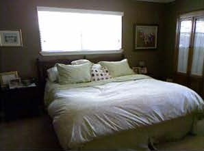
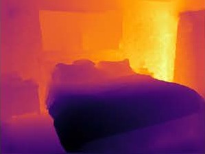
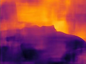
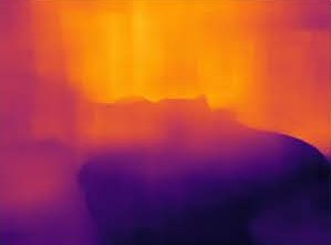
| Input | Ground Truth | Baseline | Method |
|---|---|---|---|
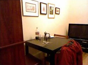 | 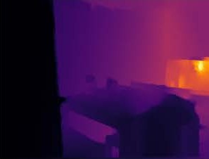 | 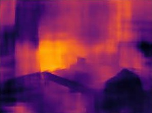 | 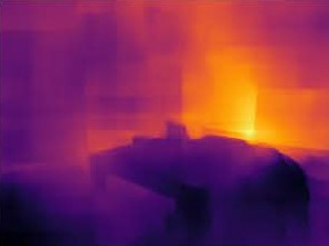 |
 |  |  |  |
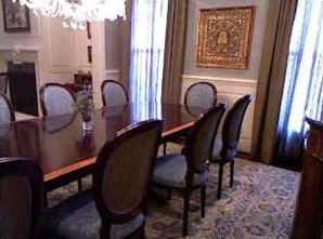 | 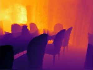 | 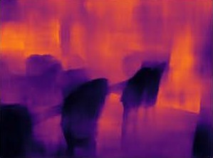 | 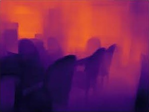 |
Summary:
- Lower MSE and higher SSIM than the baseline, despite a much shallower network
- \(\sim 14 \times\) fewer parameters than the baseline U-Net
- \(\sim 6 \times\) faster inference, reaching \(35.5\) FPS — meeting real-time requirements (typically defined as \(24–30\) FPS)
- Qualitative results showed better object boundary accuracy and continuity in low-frequency regions compared to the baseline (e.g., tables, beds, sofas, chairs)
Future Improvements
- Improve prediction accuracy for smaller and stacked/cluttered objects
- Improve handling of transparent and reflective materials
- Integrate the network into a full video depth mapping pipeline to evaluate real-world inference speed in practice
References
Contact
Aniket Patil
GitHub @AniketP04 · LinkedIn · aniketkolte0406@gmail.com
Open a GitHub Issue for bugs, questions, or feature requests.