Pixels from the Void: A Deep Technical Comparison of Upsampling Methods in Monocular Depth Estimation and Dense Prediction Networks

Pixels from the Void: A Deep Technical Comparison of Upsampling Methods in Monocular Depth Estimation and Dense Prediction Networks

1. Introduction: Why Upsampling Is the Silent Bottleneck

Modern deep learning architectures for dense prediction tasks — monocular depth estimation, semantic segmentation, optical flow, surface normal estimation, and stereo disparity — all share a fundamental architectural tension: the spatial compression-decompression problem. Convolutional neural networks are extraordinarily good at distilling high-resolution visual signals into compact, semantically rich latent representations. But what goes in at full resolution must come out at full resolution, and the path from abstract feature maps back to dense pixel-level predictions is where quality is often won or lost.

Consider monocular depth estimation: given a single RGB image, the network must predict a per-pixel depth value that captures precise geometric structure — the exact boundary where a wall meets a floor, the smooth curvature of a distant hill, the sharp edge of a windowsill. These demands are simultaneously high-frequency (sharp edges, discontinuities) and low-frequency (smooth planar surfaces, gradual depth gradients). No single upsampling method excels at both simultaneously, and the choice of upsampling strategy propagates through the decoder in ways that are non-obvious until you observe failure modes in the wild.

The Spatial Resolution Collapse Problem

In a standard CNN encoder (VGG, ResNet, EfficientNet, or a Vision Transformer with patch embeddings), spatial resolution is progressively reduced by strided convolutions or pooling layers. A common encoder reduces a $640×192$ input to a $20×6$ feature map at the bottleneck — a $32×$ spatial compression factor. Each downsampling step doubles the receptive field but halves spatial resolution, trading positional precision for semantic abstraction.

The decoder’s job is to invert this process. But this inversion is fundamentally ill-posed: spatial detail destroyed in the encoder cannot be recovered from the feature maps alone. This is why skip connections (as in U-Net and FPN-style architectures) are so critical — they bypass the bottleneck entirely, fusing high-resolution early-encoder features with semantically rich late-encoder features at each decoder stage.

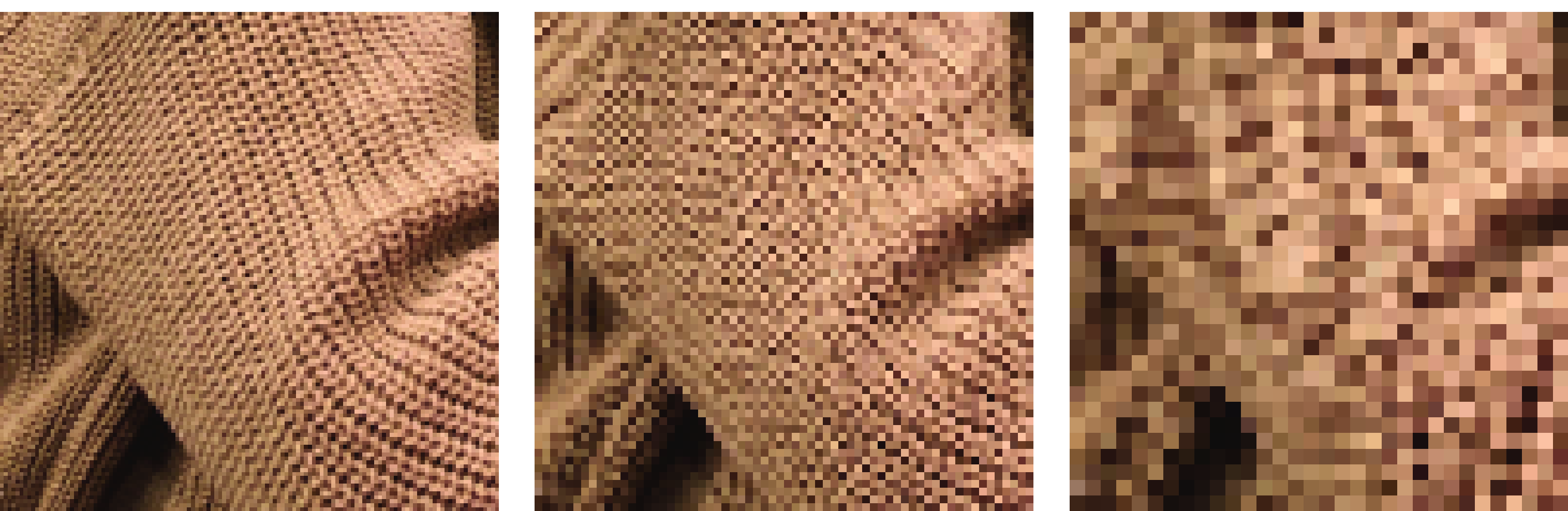
The upsampling operator sits at the core of each decoder stage, determining how feature maps transition between resolutions. The choice of upsampling method governs:

Artifact structure: are the upsampling artifacts regular (checkerboard) or diffuse (blur)?
Gradient flow: does the upsampling have learnable parameters that participate in backpropagation?
Frequency behavior: does the method suppress, preserve, or amplify high-frequency spatial information?
Computational cost: does the upsampling operator scale with the number of channels and output resolution?

Why Depth Estimation Is Especially Sensitive

Depth estimation is among the hardest dense prediction tasks to upsample well, for reasons that compound:

Depth discontinuities at object boundaries require sharp, localized transitions — but oversmoothing from bilinear interpolation softens these transitions, producing “depth bleeding” where foreground object depth bleeds into background regions.
Smooth planar surfaces (walls, floors, roads) require spatially consistent, artifact-free predictions. Checkerboard artifacts from improperly configured transposed convolutions produce sinusoidal ripples on planar surfaces — artifacts that are visually obvious and geometrically nonsensical.
Self-supervised depth training uses photometric reprojection losses that are extremely sensitive to spatial structure. Artifacts in the predicted depth map produce systematic photometric errors that reinforce themselves during training.
Downstream applications — 3D reconstruction, SLAM, robotics, autonomous driving — amplify any upsampling artifacts into geometric errors that accumulate in the scene representation.

The decoder is not a solved problem. Understanding the mechanics and tradeoffs of each upsampling method is essential for designing systems that work at the edge of what the state-of-the-art demands.

2. What Is Upsampling, Formally?

Upsampling, in the context of neural network decoders, is the operation that maps a feature tensor of spatial dimensions $(H, W)$ to a larger tensor of spatial dimensions $(sH, sW)$ where $s > 1$ is the scale factor. For integer scale factors, the operation is called upsampling; for non-integer scale factors, it is more generally called spatial interpolation.

Formally, given an input feature map $F \in \mathbb{R}^{C \times H \times W}$, the upsampling operation $\mathcal{U}: \mathbb{R}^{C \times H \times W} \to \mathbb{R}^{C \times H' \times W'}$ produces an output $F' \in \mathbb{R}^{C \times H' \times W'}$ where $H' = sH$ and $W' = sW$.

The key design choices are:

Interpolation strategy: how are values at new grid positions computed from existing values?
Learnability: does the operation have parameters optimized during training?
Independence: is the same operation applied channel-by-channel, or is there cross-channel mixing?

In encoder-decoder depth architectures, a typical decoder performs a sequence of upsampling stages:

Bottleneck (20×6, 512 channels)
    → Upsample ×2 → Conv → (40×12, 256 channels)
    → Upsample ×2 → Conv → (80×24, 128 channels)
    → Upsample ×2 → Conv → (160×48, 64 channels)
    → Upsample ×2 → Conv → (320×96, 32 channels)
    → Upsample ×2 → Conv → (640×192, 1 channel) [depth map]

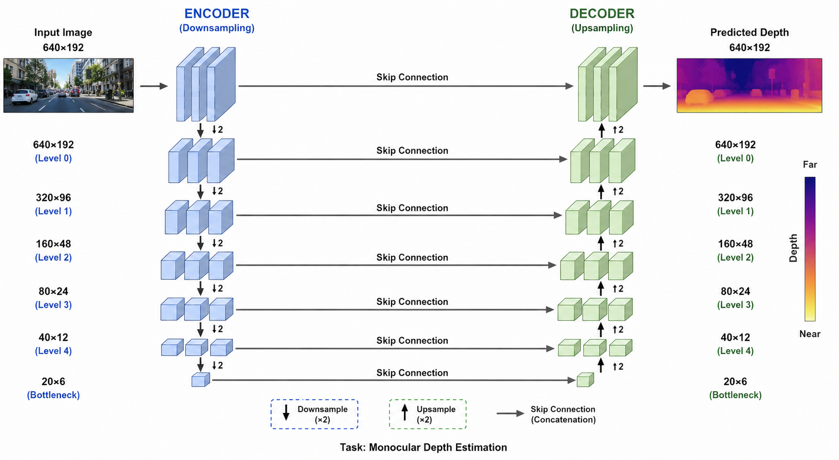
Each upsampling step doubles spatial resolution, and at each step the choice of upsampling method shapes the quality of the reconstructed feature maps that subsequent convolutions operate on.

3. Nearest Neighbor Upsampling

Mathematical Mechanics

Nearest neighbor upsampling is the simplest possible spatial interpolation: to assign a value to a new grid position, find the nearest input grid position and copy its value exactly.

For an input feature map of size $H \times W$ being upsampled to $H' \times W'$ with integer scale factor $s$, the mapping is:

\[F'[i, j] = F\left[\left\lfloor \frac{i}{s} \right\rfloor, \left\lfloor \frac{j}{s} \right\rfloor\right]\]

This is pixel replication. Each input pixel is expanded into an $s \times s$ block of identical values. The mapping is purely spatial — no mixing of values from neighboring pixels occurs.

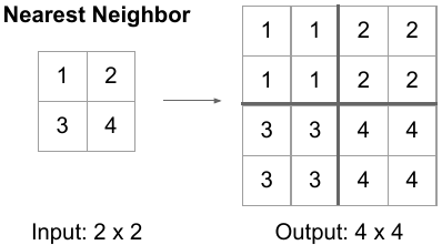
The coordinate mapping is discrete: each output pixel maps to exactly one input pixel, with no fractional contributions. This makes nearest neighbor discontinuous — the transition between adjacent blocks is a sharp step function.

Implementation

In PyTorch, nearest neighbor upsampling is accessed via:

import torch
import torch.nn as nn
import torch.nn.functional as F

upsampled = F.interpolate(features, scale_factor=2, mode='nearest')

upsample_nn = nn.Upsample(scale_factor=2, mode='nearest')
output = upsample_nn(features)  # features: (B, C, H, W)

A typical decoder block using nearest neighbor:

class NearestNeighborDecoder(nn.Module):
    def __init__(self, in_channels, out_channels):
        super().__init__()
        self.upsample = nn.Upsample(scale_factor=2, mode='nearest')
        self.conv = nn.Sequential(
            nn.Conv2d(in_channels, out_channels, 3, padding=1),
            nn.BatchNorm2d(out_channels),
            nn.ReLU(inplace=True)
        )

    def forward(self, x, skip=None):
        x = self.upsample(x)
        if skip is not None:
            x = torch.cat([x, skip], dim=1)
        return self.conv(x)

The nearest neighbor upsample has zero learnable parameters and is implemented as a simple memory gather operation.

Computational Characteristics

FLOPs: Effectively zero — each output element requires a single memory read with no arithmetic.
Memory: Output tensor is $s^2$ times larger than input; peak memory is dominated by I/O.
Cache behavior: Memory access patterns are regular and predictable — highly cache-friendly.
Hardware efficiency: Nearest neighbor maps trivially to vectorized gather operations, making it extremely fast on GPUs and mobile hardware alike.

For an input of size $C \times H \times W$ at scale factor $s = 2$: the output has $C \times 4HW$ elements, each requiring exactly one memory access with no multiply-accumulate operations.

Artifacts and Failure Modes

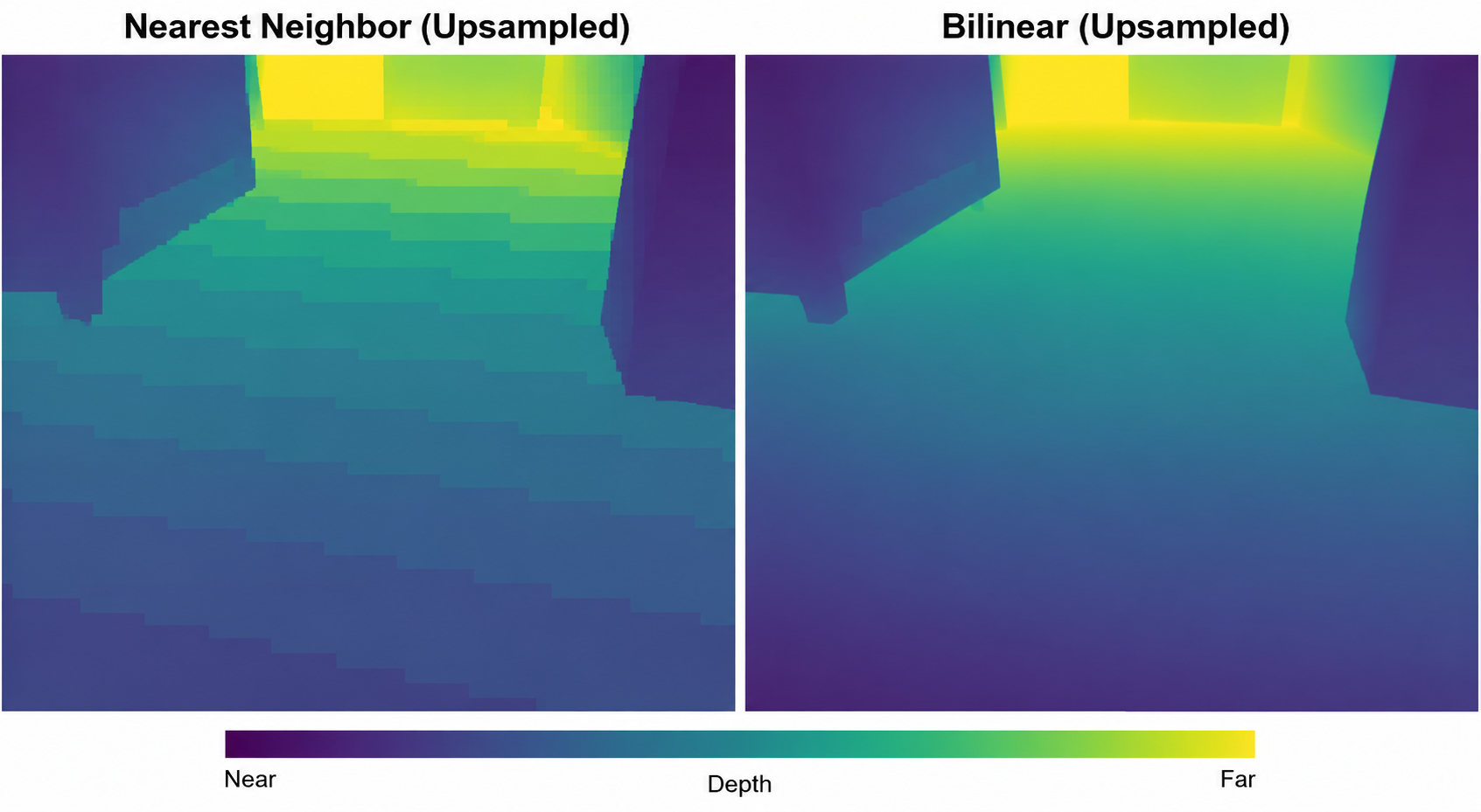
The fundamental problem with nearest neighbor upsampling is immediately apparent in any visualization: blocky artifacts. Because values are replicated rather than interpolated, spatial boundaries in the feature map appear as rectangular blocks in the output, regardless of the true object boundary orientation.

For depth estimation specifically:

Jagged depth edges: Boundaries between objects become staircase patterns, especially visible on diagonal edges. A wall at $45°$ to the image plane produces a staircase depth discontinuity rather than a clean line.
Block frequency injection: The $s \times s$ replication pattern introduces artificial spatial frequencies at $f = \frac{1}{(s \cdot \text{pixel_size})}$ into the feature maps. Subsequent convolutions partially suppress these, but cannot eliminate them entirely.
Poor surface reconstruction: Smooth, gradually varying surfaces (a receding floor, a curved object) show visible terracing — discrete depth steps corresponding to the upsampling block size.

When to Use Nearest Neighbor

Despite its limitations, nearest neighbor upsampling is genuinely useful in specific contexts:

Semantic segmentation with hard class boundaries: when you ultimately apply an argmax over class logits, spatial smoothness of intermediate feature maps matters less. The final argmax introduces its own hard discontinuities.
Lightweight and mobile architectures: when decoder computational budget is severely constrained, the overhead savings of nearest neighbor vs. bilinear are meaningful. MobileNet-based segmentation models often use nearest neighbor for this reason.
Label propagation and mask upsampling: when upsampling discrete segmentation labels or binary masks (not continuous feature maps), nearest neighbor is correct — you do not want to interpolate between class labels.
Real-time systems where latency is critical and artifact suppression is handled downstream by a refinement step.

4. Bilinear Upsampling

Mathematical Mechanics

Bilinear interpolation extends the 1D linear interpolation concept to 2D: a value at a continuous coordinate $(x, y)$ is estimated as the weighted sum of its four nearest integer-grid neighbors, with weights proportional to proximity.

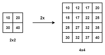
For an output position $(i', j')$ in the upsampled grid, the corresponding input coordinate is:

\[x = \frac{i'}{s}, \quad y = \frac{j'}{s}\]

The four nearest integer-grid input positions are:

\[x_0 = \lfloor x \rfloor, \quad x_1 = x_0 + 1, \quad y_0 = \lfloor y \rfloor, \quad y_1 = y_0 + 1\]

The fractional distances are:

\[\alpha = x - x_0, \quad \beta = y - y_0\]

The bilinear interpolation formula is:

\[F'[i', j'] = (1-\alpha)(1-\beta)\, F[x_0, y_0] + \alpha(1-\beta)\, F[x_1, y_0] + (1-\alpha)\beta\, F[x_0, y_1] + \alpha\beta\, F[x_1, y_1]\]

This can be seen as two nested linear interpolations: first along the $x$-axis at both $y_0$ and $y_1$, then linearly combining the results along the $y$-axis.

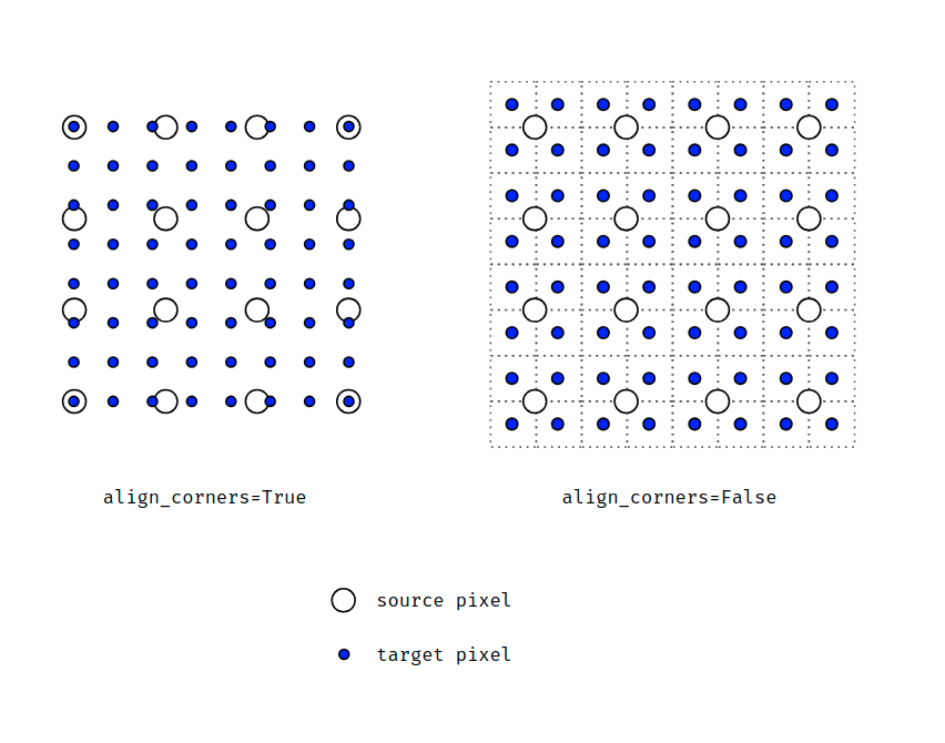
For a scale factor of $s = 2$ with align_corners=False (PyTorch default), the input coordinates of the output pixels are:

Output pixel	Input coord
0	0.25
1	0.75
2	1.25
3	1.75

With align_corners=True, the input corners align exactly with output corners:

Output pixel	Input coord
0	0.0
1	0.333
2	0.667
3	1.0

The difference becomes significant at borders and for downstream geometric operations — particularly relevant in depth estimation when converting depth maps to 3D point clouds or computing homographies.

Smoothness and Gradient Properties

The bilinear interpolation function is $C^0$ continuous (continuous but not differentiable everywhere) — it is piecewise-linear, with kinks at the input grid boundaries. This is a critical property:

The interpolated function is smooth within each cell but has discontinuous first derivatives at cell boundaries.
In the context of depth estimation, this means bilinear upsampling produces smooth gradients within regions but may introduce subtle artifacts at input grid positions.

From a training perspective, bilinear upsampling has a well-defined gradient with respect to its inputs (used during backpropagation) even though it has no learnable parameters:

\[\frac{\partial \mathcal{L}}{\partial F[x_0, y_0]} = \sum_{(i', j') \to (x_0, y_0)} (1-\alpha)(1-\beta) \frac{\partial \mathcal{L}}{\partial F'[i', j']}\]

The gradient accumulates from all output positions that interpolate from the same input position, weighted by the same bilinear coefficients used in the forward pass. This makes bilinear upsampling a well-behaved operation in computation graphs.

Implementation

import torch
import torch.nn as nn
import torch.nn.functional as F

# align_corners behavior matters
upsampled_default = F.interpolate(
    features, scale_factor=2, mode='bilinear', align_corners=False
)
upsampled_aligned = F.interpolate(
    features, scale_factor=2, mode='bilinear', align_corners=True
)

# bilinear upsample + refining convolution
class BilinearDecoder(nn.Module):
    def __init__(self, in_channels, out_channels, skip_channels=0):
        super().__init__()
        self.upsample = nn.Upsample(
            scale_factor=2, mode='bilinear', align_corners=False
        )
        self.conv = nn.Sequential(
            nn.Conv2d(in_channels + skip_channels, out_channels, 3, padding=1),
            nn.ELU(inplace=True),
            nn.Conv2d(out_channels, out_channels, 3, padding=1),
            nn.ELU(inplace=True),
        )

    def forward(self, x, skip=None):
        x = self.upsample(x)
        if skip is not None:
            x = torch.cat([x, skip], dim=1)
        return self.conv(x)

This upsample + convolution pattern — often called resize-convolution — is the dominant paradigm in modern depth decoders. The convolution following the upsample learns to refine the smooth upsampled features, recovering high-frequency detail that bilinear interpolation alone cannot reconstruct.

Why Bilinear Became the Default in Depth Estimation

Several factors converged to make bilinear upsampling dominant:

1. Artifact-free smooth surfaces. Monodepth2, which introduced the multi-scale self-supervised depth framework, deliberately replaced transposed convolutions with bilinear upsampling precisely to eliminate checkerboard artifacts that degraded photometric reprojection losses on smooth surfaces. The paper observed that checkerboard artifacts produced systematic photometric errors on walls, floors, and ceilings — exactly the regions that drive the depth network to learn geometric structure.

2. Stable self-supervised training. Photometric loss functions based on SSIM and L1 error between reprojected and reference frames are sensitive to high-frequency noise. Bilinear upsampling’s smoothness suppresses artifact frequencies that would otherwise create spurious training signal.

3. Compatibility with modern encoders. As encoders grew stronger (ViT, Swin Transformer, ConvNeXt), the decoder’s role shifted toward feature fusion rather than spatial reconstruction. Strong encoders with skip connections reduce the decoder’s burden, making simple but clean bilinear upsampling sufficient.

4. MiDaS and DPT architecture. MiDaS and its successor DPT — which achieve state-of-the-art monocular depth on diverse datasets — use bilinear interpolation in their feature pyramid decoders. DPT reassembles ViT tokens into dense feature maps using bilinear upsampling between resolution stages, demonstrating that learned encoders can compensate for the smoothness limitations of fixed-weight upsampling.

Computational Characteristics

For an input of shape $C \times H \times W$ upsampled by factor $s$:

FLOPs: Each output pixel requires 4 multiplications and 3 additions (bilinear combination of 4 neighbors). Total: $7 \times C \times s^2 \times H \times W$ operations.
Memory: Output is $s^2$ times larger; intermediate computations are minimal.
GPU efficiency: Bilinear interpolation is natively supported in CUDA and maps efficiently to texture memory hardware. Modern GPUs implement bilinear sampling in dedicated texture units that are separate from CUDA cores — making it effectively “free” in terms of shader occupancy.
Cache behavior: Access to 4 neighboring input pixels per output pixel is cache-friendly for small feature maps but may cause cache pressure at high resolutions.

Failure Modes

Despite its advantages, bilinear upsampling has documented failure modes in depth estimation:

Oversmoothing at depth discontinuities: Bilinear interpolation is a low-pass filter. Sharp depth transitions (object boundaries, occlusion edges) are systematically smoothed, producing halos and depth bleed. This becomes critical in applications requiring precise 3D geometry for robotic manipulation or autonomous driving collision avoidance.
Texture-less region ambiguity: In regions where the encoder features themselves are smooth, bilinear upsampling cannot recover fine-grained depth structure — the information simply isn’t in the feature map.
Scale inconsistency at borders: The align_corners parameter changes the effective coordinate mapping, which can introduce subtle boundary inconsistencies when combining features at different scales (especially in FPN-style decoders).

5. Transposed Convolution (Deconvolution)

Conceptual Foundation

Transposed convolution — also called fractionally strided convolution or, imprecisely, deconvolution — is the most powerful and most dangerous upsampling method. Unlike interpolation-based approaches that apply a fixed mathematical formula, transposed convolution learns its upsampling kernel from data, enabling the decoder to synthesize spatially detailed feature maps that no fixed interpolation could reconstruct.

The name “transposed convolution” comes from the relationship to standard convolution expressed as a matrix multiplication. A standard convolution with kernel $K$, stride $s$, and input $x$ can be written as:

\[y = C_K \cdot x\]

where $C_K$ is a sparse Toeplitz matrix derived from $K$. The transposed convolution applies $C_K^T$:

\[y = C_K^T \cdot x\]

This matrix transpose reverses the spatial mapping: where standard convolution maps $N$ input positions to $M < N$ output positions (with stride $> 1$), transposed convolution maps $M$ input positions to $N > M$ output positions. The operator is the gradient of the standard convolution with respect to its input — which is why transposed convolution appears naturally in backpropagation through convolutional layers.

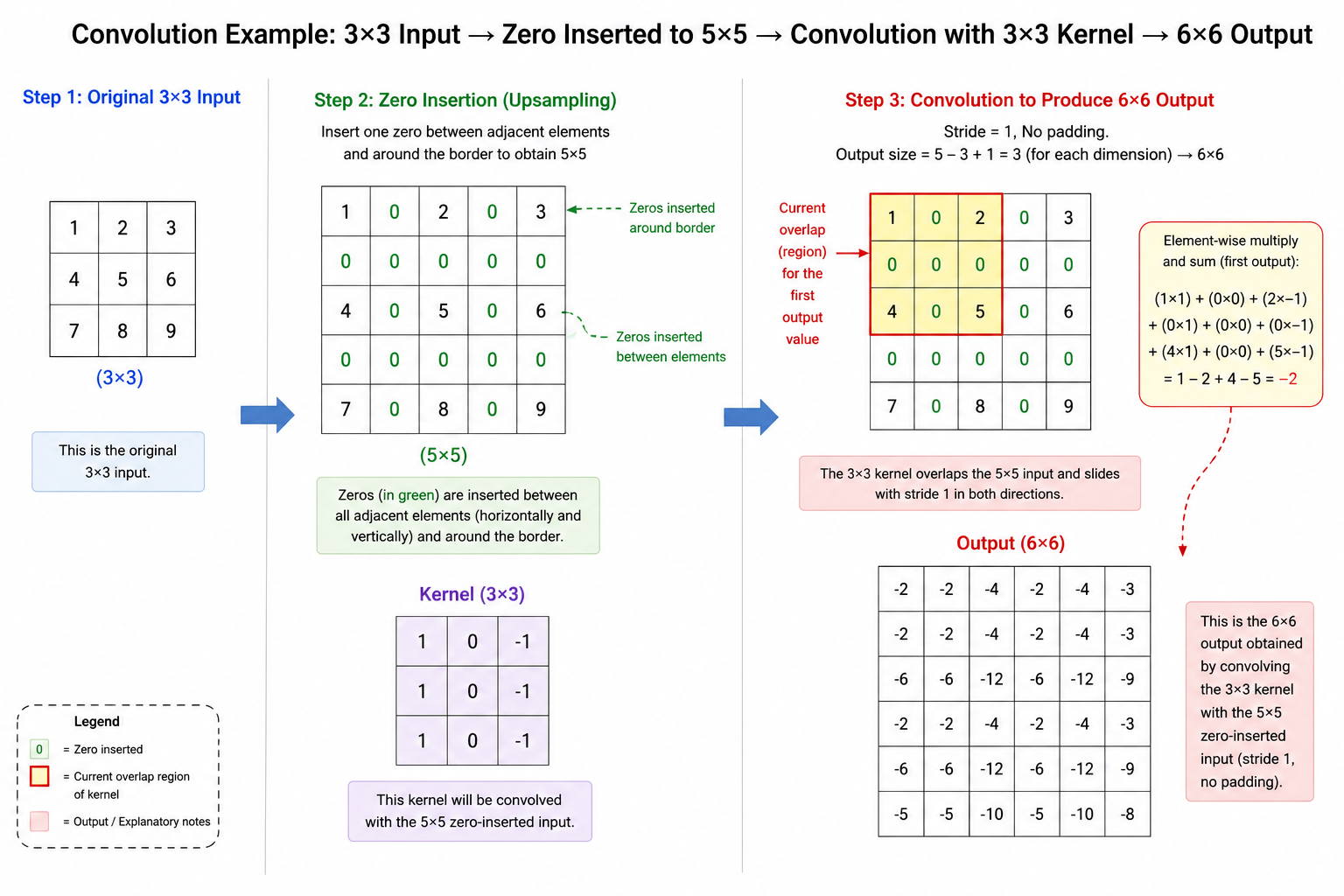
Mechanics: Zero Insertion and Kernel Sliding

The practical implementation of transposed convolution proceeds as follows:

Insert zeros: Between each pair of input pixels, insert $s - 1$ rows/columns of zeros, expanding the input from $H \times W$ to $(H + (H-1)(s-1)) \times (W + (W-1)(s-1))$.
Pad the expanded input: Apply padding $p' = k - 1 - p$ (where $k$ is kernel size and $p$ is the original convolution padding).
Apply standard convolution (stride 1) to the padded expanded input.

For input size $H \times W$, kernel size $k$, stride $s$, and padding $p$, the output size is:

\[H' = (H - 1) \cdot s - 2p + k\]

With $k = 4$, $s = 2$, $p = 1$: $H' = (H-1) \cdot 2 - 2 + 4 = 2H$. This doubles spatial resolution, the standard decoder use case.

Implementation

import torch
import torch.nn as nn

# basic transposed convolution upsampling
transposed_conv = nn.ConvTranspose2d(
    in_channels=256,
    out_channels=128,
    kernel_size=4,  
    stride=2,
    padding=1
)

# With correct kernel size: k=4, s=2, p=1 → doubles resolution
# output_size = (H-1)*2 - 2*1 + 4 = 2H

# anti-checkerboard pattern: k=4, s=2 (k divisible by s)
class DeconvDecoder(nn.Module):
    def __init__(self, in_channels, out_channels):
        super().__init__()
        self.deconv = nn.ConvTranspose2d(
            in_channels, out_channels, kernel_size=4, stride=2, padding=1
        )
        self.bn = nn.BatchNorm2d(out_channels)
        self.relu = nn.ReLU(inplace=True)

    def forward(self, x, skip=None):
        x = self.relu(self.bn(self.deconv(x)))
        if skip is not None:
            x = torch.cat([x, skip], dim=1)
        return x

Parameters and Computational Cost

For a transposed convolution with $C_{in}$ input channels, $C_{out}$ output channels, and $k \times k$ kernel:

Parameters: $C_{in} \times C_{out} \times k^2 + C_{out}$ (with bias)
FLOPs: $C_{in} \times C_{out} \times k^2 \times H' \times W'$

For comparison: a bilinear upsample followed by a $3 \times 3$ convolution on the same channels has:

Parameters: $C_{in} \times C_{out} \times 9$
FLOPs: $C_{in} \times C_{out} \times 9 \times H' \times W'$

Asymptotically, transposed convolution and resize-convolution have similar FLOPs for equivalent kernel sizes. The critical difference is that transposed convolution performs upsampling and feature transformation in a single fused operation, while resize-convolution separates them.

The Checkerboard Artifact Problem

Checkerboard artifacts are the most significant failure mode of transposed convolution, and their origin is mathematical rather than implementation-dependent.

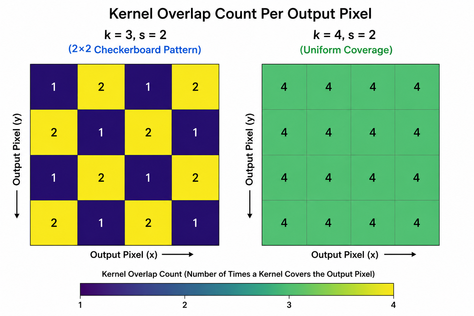
The root cause is uneven kernel overlap. When a transposed convolution kernel slides over the zero-inserted input, different output positions receive contributions from different numbers of kernel coefficients, depending on their alignment with the kernel stride pattern.

For kernel size $k = 3$, stride $s = 2$: the kernel divides into two groups of coefficients — those at even positions and those at odd positions relative to the stride. Some output pixels receive contributions from 4 kernel weights, others from 2 or 1. This non-uniform coverage creates a spatially periodic pattern in the output whose frequency is $\frac{1}{s}$ — a checkerboard at the stride period.

Formally, define the output pixel position $(i, j)$ modulo the stride $s$:

\[n_{ij} = |\{(k_x, k_y) : (i - k_x) \equiv 0 \pmod{s}, (j - k_y) \equiv 0 \pmod{s}, 0 \le k_x, k_y < k\}|\]

When $k$ is not divisible by $s$, $n_{ij}$ varies across positions $(i, j)$, creating the spatially non-uniform contribution pattern that produces checkerboards.

The fix is to choose kernel size $k$ divisible by stride $$s$ (e.g., $k = 4$ for $s = 2$). With $k = 4$, $s = 2$: every output position receives contributions from exactly 4 kernel coefficients at positions $(0,0), (0,2), (2,0), (2,2)$ relative to the kernel center — uniform coverage, no checkerboard.

Checkerboard artifacts in depth estimation are particularly damaging because:

Planar surface violation: Walls, floors, and ceilings should have nearly-constant depth. A checkerboard pattern on these surfaces produces physically impossible oscillating depth values.
Photometric loss amplification: In self-supervised training, these geometric oscillations appear as systematic photometric inconsistencies, creating a feedback loop that reinforces the artifact pattern.
3D reconstruction corruption: When the depth map feeds a 3D reconstruction pipeline (NeRF, SLAM, MVS), checkerboard artifacts create ghost geometry that poisons the scene representation.

Mitigation Strategies

Beyond choosing $k$ divisible by $s$, several approaches have been developed:

1. Resize-Convolution: Replace transposed convolution with nearest-neighbor or bilinear upsample followed by standard convolution. The standard convolution has uniform receptive field coverage, eliminating uneven overlap. This is now the dominant paradigm.

2. Sub-pixel Convolution: Perform a standard convolution to produce $C \times s^2$ channels, then rearrange (pixel shuffle) to produce $C$ channels at $s \times$ resolution. Sub-pixel convolution has uniform overlap (no zero insertion) and is popular in super-resolution networks.

# sub-pixel convolution (PixelShuffle)
class SubPixelUpsample(nn.Module):
    def __init__(self, in_channels, out_channels, scale_factor=2):
        super().__init__()
        self.conv = nn.Conv2d(in_channels, out_channels * scale_factor**2, 3, padding=1)
        self.shuffle = nn.PixelShuffle(scale_factor)

    def forward(self, x):
        return self.shuffle(self.conv(x))

3. Refinement Blocks: Apply transposed convolution followed by a standard $3 \times 3$ convolution (or group-norm + activation + conv) to suppress residual artifacts.

4. Guided Upsampling: Upsample depth features guided by high-resolution RGB features using bilateral filtering or learned guidance kernels (CARAFE, SAPA).

6. Why Modern Depth Estimation Prefers Bilinear Upsampling

The shift from transposed convolution to bilinear upsampling in depth estimation decoders was not arbitrary — it reflects a deeper architectural insight about where representational capacity should be invested.

The Encoder Dominance Principle

In early encoder-decoder depth architectures (DispNet, early DepthNet variants), the encoder was relatively weak (VGG-based), and the decoder was expected to contribute substantially to depth quality through learned upsampling. Transposed convolutions were favored because their learnable kernels could synthesize spatial detail that weak encoders failed to preserve.

As encoders grew stronger — ResNet, EfficientNet, Swin Transformer, ViT — the depth of encoder feature representations exploded, and the decoder’s role became primarily one of feature fusion and resolution restoration rather than detail synthesis. The information needed to reconstruct a sharp depth map is present in the encoder’s skip-connection features; the decoder’s job is to fuse it correctly, not to hallucinate it from scratch.

This shift made fixed, clean bilinear upsampling more attractive: it provides a neutral, artifact-free spatial canvas onto which skip-connection features can be fused and refined by subsequent convolutions.

The Monodepth2 Inflection Point

Monodepth2 crystallized this shift in the self-supervised depth community. Its decoder is structurally simple: bilinear upsample, then a pair of $3 \times 3$ convolutions with ELU activations. No transposed convolutions appear anywhere in the decoder. The decoder is deliberately weak, with most representational capacity concentrated in the ResNet encoder and the multi-scale photometric loss design.

The multi-scale prediction strategy — producing depth maps at $\frac{1}{1}$, $\frac{1}{2}$, $\frac{1}{4}$, and $\frac{1}{8}$ resolution during training — further reduces the decoder’s burden: each scale only needs to upsample by $2 \times$ at most before producing a loss signal.

DPT and Transformer Decoders

DPT (Dense Prediction Transformer) exemplifies the modern extreme of encoder dominance. The decoder is a feature pyramid that reassembles ViT patch tokens at multiple resolutions, combining them with learned projections and bilinear upsampling. The ViT encoder, pretrained on large-scale datasets, encodes all necessary spatial detail; the decoder’s bilinear upsampling is essentially a coordinate transformation rather than a representational bottleneck.

Similarly, Depth Anything and ZoeDepth follow the same paradigm: powerful encoder (DINOv2 or BEiT), simple decoder with bilinear upsampling and lightweight refinement convolutions.

Where Transposed Convolution Remains Valuable

Despite the trend, transposed convolution retains niches:

Generative models (VAE decoders, conditional GANs for depth completion): when the decoder must synthesize detail with no skip connections, learned upsampling is critical.
Depth completion (sparse LiDAR + RGB): the decoder must reconstruct full-resolution depth from sparse guidance, a synthesis task where learned upsampling outperforms interpolation.
Compact models without skip connections: when memory constraints prohibit skip connections, transposed convolution compensates.

7. Computational and Deployment Considerations

GPU Efficiency

Bilinear upsampling maps to CUDA texture sampling hardware, which operates asynchronously from the shader core pipeline. On NVIDIA GPUs, texture operations are handled by dedicated TMUs (Texture Mapping Units), meaning bilinear upsampling consumes essentially zero shader occupancy. This is a strong practical advantage in decode-heavy pipelines.

Nearest neighbor maps to trivial gather operations — equally efficient, slightly less flexible in its coordinate handling.

Transposed convolution maps to matrix multiplication (GEMM), which is the most GPU-efficient operation type on tensor core hardware but requires careful channel sizing to achieve full tensor core utilization. Transposed convolutions with channel counts that are not multiples of 8 (FP16) or 16 (INT8) fail to use tensor cores efficiently.

Mobile and Edge Deployment

For mobile deployment (iOS CoreML, Android NNAPI, TFLite), the support and optimization level varies:

Nearest neighbor: universally supported, highly optimized on all mobile hardware.
Bilinear: widely supported; the align_corners parameter must be handled carefully when converting between frameworks (ONNX → TFLite conversions have historically introduced alignment bugs).
Transposed convolution: supported but less optimized on mobile NPUs. Some edge NPU compilers (e.g., TI DSP, Qualcomm SNPE) have limited or buggy transposed convolution support and perform better with explicit resize-convolution patterns.

For autonomous driving inference on embedded platforms (NVIDIA Jetson, Hailo, Mobileye), bilinear upsampling is the safest choice from a toolchain compatibility perspective.

Real-Time SLAM and Robotics

Monocular depth models deployed in SLAM pipelines (DepthSLAM, DROID-SLAM) require predictable, temporally consistent depth maps. Nearest neighbor upsampling can produce temporal flickering at block boundaries when features change between frames. Bilinear upsampling’s smooth interpolation reduces temporal noise. Transposed convolution, if undertrained or with artifact patterns, can produce per-frame checkerboard oscillations that break pose estimation.

8. Practical Recommendations

When to Use Nearest Neighbor

Use nearest neighbor when:

Deploying on severely resource-constrained hardware where every operation counts (MCU-class devices, DSP inference with minimal FLOP budgets).
Upsampling discrete labels or masks — never interpolate between class IDs.
As a stepping stone in lightweight architectures where subsequent convolutions are expected to suppress artifacts (e.g., MobileNetV3 segmentation decoders).
In research ablations to establish a computational lower bound on decoder quality.

Avoid nearest neighbor for monocular depth estimation where output quality is important, for any geometry-sensitive application, or where temporal consistency across frames is required.

When to Use Bilinear

Use bilinear upsampling as your default in nearly all depth estimation and dense prediction systems:

Self-supervised monocular depth (Monodepth2-style): bilinear + convolution is the correct choice, essentially unconditionally.
Transformer-based depth decoders (DPT, Depth Anything): the decoder’s role is feature fusion, not synthesis; bilinear provides a clean spatial canvas.
Production systems with cross-platform deployment: bilinear is universally supported and optimized.
Indoor depth estimation: smooth surfaces dominate; bilinear’s smoothness is a feature, not a bug.
Any system using photometric or perceptual losses: bilinear avoids artifact-driven spurious loss signals.

Be cautious with bilinear when the task demands precise depth boundary sharpness (robotic grasping, collision avoidance), or when working with textureless regions where the encoder features themselves are smooth — in these cases, add a dedicated edge-preserving refinement module (detail transfer from RGB, guided filtering).

When to Use Transposed Convolution

Use transposed convolution when:

The decoder must synthesize detail without skip connections (depth completion from sparse LiDAR, depth prediction in generative pipelines).
You have strong decoder supervision (full-resolution ground truth at every decoder stage) that prevents artifact reinforcement.
You need maximum theoretical output quality in a research setting where inference speed is not the primary constraint.
Sub-pixel convolution (PixelShuffle) is an attractive alternative in the same regime with better artifact properties.

Always use $k$ divisible by $s$ ($k = 4$, $s = 2$ is the standard safe choice). If you observe checkerboard artifacts, immediately switch to resize-convolution.

9. Conclusion: Engineering Beyond the Obvious Choice

There is no universally optimal upsampling method for depth estimation or dense prediction — there is only the best method for a given combination of encoder strength, decoder structure, loss function, deployment target, and output quality requirements.

The trajectory of monocular depth estimation architectures tells an instructive story. Early networks invested heavily in learned transposed convolution decoders, compensating for weak encoders. As encoder representations strengthened through scale and pretraining, the decoder’s role diminished, and bilinear upsampling emerged as the dominant choice — not because it is the most capable method, but because it is the cleanest: artifact-free, stable in training, efficient in deployment, and sufficient when paired with powerful encoders and well-designed skip connections.

Transposed convolution retains genuine value in contexts where the decoder must do real representational work — but it should be used with full awareness of its failure modes and mitigated with proper kernel-stride design or replaced with sub-pixel convolution where artifacts are unacceptable.

Nearest neighbor remains useful precisely at the margins: discrete label upsampling, ultra-lightweight models, and as a fast-path in systems where downstream refinement absorbs its artifacts.

The deeper engineering insight is that upsampling method selection is inseparable from the rest of the system design. The choice ripples through encoder design (how strong must it be?), skip connection design (what detail can be recovered from early features?), loss function design (how sensitive is the training signal to spatial artifacts?), and deployment design (what operations are optimized on the target hardware?).

The best depth estimation systems — Monodepth2, DPT, Depth Anything, ZoeDepth — do not win because of their upsampling methods. They win because their entire architecture is coherent: encoder strength, decoder simplicity, training signal quality, and upsampling smoothness are all aligned. Bilinear upsampling is the right choice in these systems not as a universal truth, but because it fits cleanly into a coherent system design philosophy.

Build systems where the upsampling method is the least interesting architectural decision. That is usually the sign that everything else is working correctly.

References

Godard, C., Mac Aodha, O., Firman, M., & Brostow, G. (2019). Digging into self-supervised monocular depth estimation. ICCV 2019. (Monodepth2)
Ranftl, R., Bochkovskiy, A., & Koltun, V. (2021). Vision Transformers for Dense Prediction. ICCV 2021. (DPT)
Ranftl, R., Lasinger, K., Hafner, D., Schindler, K., & Koltun, V. (2020). Towards Robust Monocular Depth Estimation: Mixing Datasets for Zero-shot Cross-dataset Transfer. TPAMI 2020. (MiDaS)
Odena, A., Dumoulin, V., & Olah, C. (2016). Deconvolution and Checkerboard Artifacts. Distill.
Shi, W., Caballero, J., Huszar, F., et al. (2016). Real-Time Single Image and Video Super-Resolution Using an Efficient Sub-Pixel Convolutional Neural Network. CVPR 2016.
Long, J., Shelhamer, E., & Darrell, T. (2015). Fully Convolutional Networks for Semantic Segmentation. CVPR 2015.
Ronneberger, O., Fischer, P., & Brox, T. (2015). U-Net: Convolutional Networks for Biomedical Image Segmentation. MICCAI 2015.
Yang, L., Kang, B., Huang, Z., et al. (2024). Depth Anything: Unleashing the Power of Large-Scale Unlabeled Data. CVPR 2024.
Bhat, S. F., Birkl, R., Wofk, D., et al. (2023). ZoeDepth: Zero-shot Transfer by Combining Relative and Metric Depth. arXiv 2302.12288.
Wang, J., Chen, K., Xu, R., et al. (2019). CARAFE: Content-Aware ReAssembly of FEatures. ICCV 2019.

Pixels from the Void: A Deep Technical Comparison of Upsampling Methods in Monocular Depth Estimation and Dense Prediction Networks

1. Introduction: Why Upsampling Is the Silent Bottleneck

The Spatial Resolution Collapse Problem

Why Depth Estimation Is Especially Sensitive

2. What Is Upsampling, Formally?

3. Nearest Neighbor Upsampling

Mathematical Mechanics

Implementation

Computational Characteristics

Artifacts and Failure Modes

When to Use Nearest Neighbor

4. Bilinear Upsampling

Mathematical Mechanics

Smoothness and Gradient Properties

Implementation

Why Bilinear Became the Default in Depth Estimation

Computational Characteristics

Failure Modes

5. Transposed Convolution (Deconvolution)

Conceptual Foundation

Mechanics: Zero Insertion and Kernel Sliding

Implementation

Parameters and Computational Cost

The Checkerboard Artifact Problem

Mitigation Strategies

6. Why Modern Depth Estimation Prefers Bilinear Upsampling

The Encoder Dominance Principle

The Monodepth2 Inflection Point

DPT and Transformer Decoders

Where Transposed Convolution Remains Valuable

7. Computational and Deployment Considerations

GPU Efficiency

Mobile and Edge Deployment

Real-Time SLAM and Robotics

8. Practical Recommendations

When to Use Nearest Neighbor

When to Use Bilinear

When to Use Transposed Convolution

9. Conclusion: Engineering Beyond the Obvious Choice

References

Citation

Enjoy Reading This Article?