VAE-Inspired Diffusion Revolution
- Diffusion Models - Introduction
- Forward Diffusion process
- Connection with Stochastic Gradient Langevin Dynamics (SGLD)
- The Reverse Process: Learning to Denoise
- Reverse Diffusion via VAEs
- The U-Net Architecture for Noise Prediction
- Diffusion Model Algorithm
- Key Parameters in Diffusion Models
- Conclusion
- References
Diffusion Models - Introduction
Diffusion models are based on principles from non-equilibrium thermodynamics. They employ a Markov chain process that gradually injects random noise into data and subsequently learn the reverse process to generate meaningful data samples from noisy inputs. In contrast to VAE and flow-based models, diffusion models follow a predefined training procedure, and their latent variables maintain the same high dimensionality as the original data.
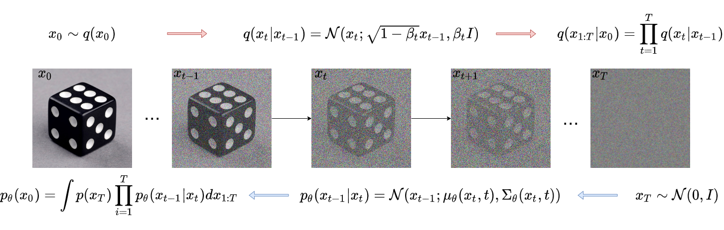
Diffusion Models are a class of generative models designed to produce data that resembles the data used during training. They operate by progressively corrupting training samples through the addition of Gaussian noise and then learning how to reconstruct the original data by reversing this noise injection process. Once trained, these models can generate new samples by transforming randomly generated noise through the learned denoising procedure.
Why not just stick with GANs?
GANs were a landmark idea — pit a generator against a discriminator and let them compete until the generator learns to fool even a sharp critic. In practice, this produces strikingly sharp images. But the adversarial setup introduces a fundamental instability: the two networks have to improve in lockstep, and if one pulls ahead, training collapses. The worst outcome is mode collapse — the generator finds a handful of outputs that reliably fool the discriminator and simply repeats them, ignoring the full diversity of the training data. You might train a GAN on thousands of distinct faces and end up with a generator that produces variations of the same three faces. Controlling what a GAN generates is also notoriously difficult; conditioning it precisely on text prompts or semantic attributes requires significant architectural gymnastics.
Why not just stick with VAEs?
VAEs solved the stability problem elegantly. Instead of a two-player game, they train a single model to compress images into a smooth latent space and reconstruct them. Training is stable and mathematically principled — you’re optimizing a proper lower bound on the data likelihood. The catch is that very stability. To ensure the latent space is smooth and continuous, the model averages over possible reconstructions. That averaging is exactly what creates blurry outputs. VAEs are great at understanding and manipulating the latent structure of data, but if you want outputs that look photographic and crisp, they fall short.
The gap that diffusion models fill.
Both failure modes — GAN instability and VAE blurriness — stem from trying to map directly between a data distribution and a latent code in one shot.
Diffusion models sidestep this entirely by breaking the generation process into many small steps. Instead of learning one big mapping, the model learns a simple operation: given a slightly noisy image, predict the noise and remove a little of it. Repeat that a few hundred times starting from pure noise, and you reconstruct a sharp, diverse image. There’s no adversarial game to destabilize training, and no compression bottleneck that forces averaged outputs. The model can capture the full multimodal richness of the training distribution — different styles, different subjects, different compositions — without collapsing or blurring them together.
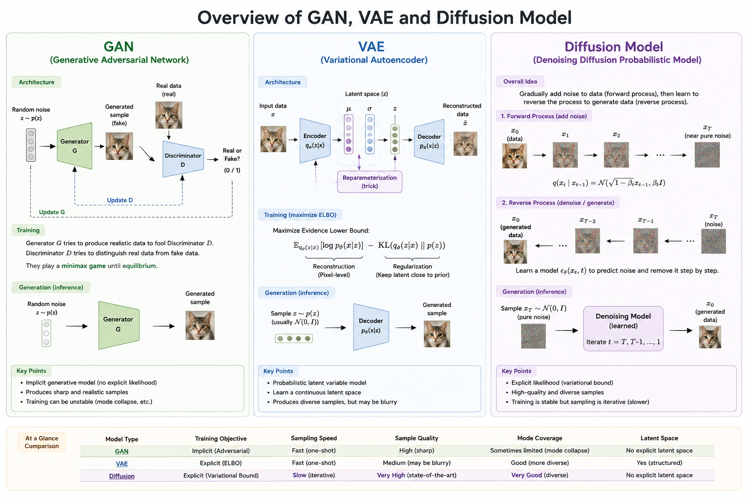
The one trade-off is speed: generating an image requires hundreds of forward passes through the network rather than one. This is an active research area, and models like DDIM and consistency models have already cut that gap significantly.
Forward Diffusion process
Given a data sample \(\mathbf{x}_0 \sim q(\mathbf{x})\) drawn from a real data distribution, a forward diffusion process is defined by gradually adding small amounts of Gaussian noise over \(T\) steps, resulting in a sequence of progressively noisier samples \(x_1,x_2,x_3,…,x_T\) .
\[\begin{aligned} q(x_t | x_{t-1}) = \mathcal{N}(x_t; \sqrt{1 - \beta_t} x_{t-1}, \beta_t I) \end{aligned}\]where:
-
\(x_t\) : the noisy image at timestep \(t\)
-
\(x_{t-1}\) : the image at the previous (less noisy) timestep
-
\(\beta_t\) : the noise schedule at timestep \(t\), controlling how much noise is added
-
\(\mathcal{N}(\mu, \sigma^2)\) : a Gaussian distribution with mean \(\mu\) and variance \(\sigma^2I\).
- Each step scales down the signal by \(\sqrt{1-\beta_t}\) (to preserve approximate unit variance) and adds Gaussian noise with variance \(\beta_t\)
The data sample \(x_0\) gradually loses its distinguishable features as the step \(t\) becomes larger. Eventually when \(T \to \infty\), \(x_T\) is equivalent to an isotropic Gaussian distribution.

A key mathematical property makes diffusion models computationally efficient: the noisy image at any timestep \(t\) can be computed directly from the original image \(x_0\), without sequentially simulating every intermediate diffusion step. This is possible because the composition of Gaussian distributions remains Gaussian.
Let \(\alpha_t = 1 - \beta_t\) and \(\bar{\alpha}_t = \prod_{i=1}^t \alpha_i\) :
\[\begin{aligned} \mathbf{x}_t &= \sqrt{\alpha_t}\mathbf{x}_{t-1} + \sqrt{1 - \alpha_t}\boldsymbol{\epsilon}_{t-1} \qquad \text{where } \boldsymbol{\epsilon}_{t-1}, \boldsymbol{\epsilon}_{t-2}, \dots \sim \mathcal{N}(\mathbf{0}, \mathbf{I}) \\[6pt] &= \sqrt{\alpha_t \alpha_{t-1}} \mathbf{x}_{t-2} + \sqrt{1 - \alpha_t \alpha_{t-1}} \,\bar{\boldsymbol{\epsilon}}_{t-2} \qquad \text{where } \bar{\boldsymbol{\epsilon}}_{t-2} \text{ merges two Gaussians} \\[6pt] &= \dots \\[6pt] &= \sqrt{\bar{\alpha}_t}\mathbf{x}_0 + \sqrt{1 - \bar{\alpha}_t}\boldsymbol{\epsilon} \\[6pt] q(\mathbf{x}_t \mid \mathbf{x}_0) &= \mathcal{N} \left( \mathbf{x}_t; \sqrt{\bar{\alpha}_t}\mathbf{x}_0, (1 - \bar{\alpha}_t)\mathbf{I} \right) \end{aligned}\](*) Recall that when we merge two Gaussians with different variance, \(\mathcal{N}(0,\sigma^2_1I)\) and \(\mathcal{N}(0,\sigma^2_1I)\), the new distribution is \(\mathcal{N}(0,(\sigma^2_1+\sigma^2_2)I)\). Here the merged standard deviation is \(\sqrt{(1 - \alpha_t) + \alpha_t (1-\alpha_{t-1})} = \sqrt{1 - \alpha_t\alpha_{t-1}}\)
The Noise Schedule
The noise schedule, denoted as \({\beta_t}_{t=1}^{T}\) determines how rapidly image structure is corrupted during the forward diffusion process. The choice of schedule plays a crucial role in the performance and quality of the diffusion model.
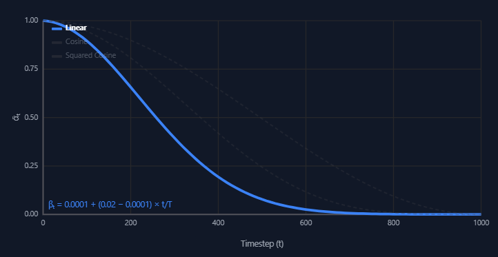
A straightforward approach is the linear schedule, where the variance term \(\beta_t\) increases linearly from a very small value (e.g., \(10^{-4}\)) to a larger value (e.g., \(0.02\)). Although intuitive, this strategy has an important limitation: it removes meaningful image structure too aggressively in the early stages, where most perceptual information is concentrated, while later timesteps spend excessive effort modeling nearly pure Gaussian noise. As a result, many denoising steps contribute little useful learning signal.

To overcome this issue, Nichol and Dhariwal introduced the cosine schedule, which defines the cumulative noise parameter \(\bar{\alpha}_t\) directly instead of specifying \(\beta_t\) indirectly:
\[\bar{\alpha}_t = \frac{f(t)}{f(0)}\]where
\[f(t)=\cos^2\left( \frac{t/T+s}{1+s}\cdot\frac{\pi}{2} \right)\]Here:
-
\(T\) is the total number of diffusion timesteps,
-
\(s\) is a small offset (typically \(0.008\)) introduced to avoid excessively large values of \(\beta_t\) near \(t=0\).
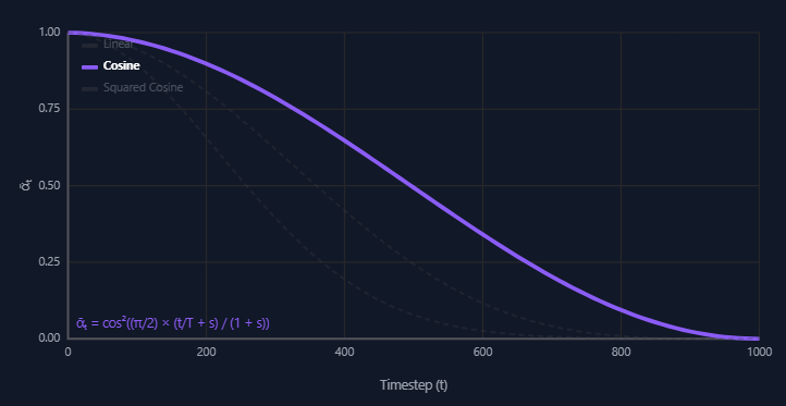
The cosine formulation causes \(\bar{\alpha}_t\) to decrease gradually from \(\mathcal{1}\) toward \(\mathcal{0}\) along a smooth cosine curve. Unlike the linear schedule, it preserves image information for a longer portion of the diffusion trajectory before progressively increasing the corruption rate. This allocates more training steps to intermediate noise levels, where the model can learn richer and more meaningful image structure.

In practice, cosine schedules consistently produce higher-quality samples than linear schedules, particularly for high-resolution image generation tasks.
More recent research has explored alternatives such as learned noise schedules, where the values of \({\beta_t}\) are optimized during training, and continuous-time diffusion models, which formulate diffusion as a stochastic differential equation rather than a discrete process. Despite these advances, linear and cosine schedules remain widely adopted because they are simple, stable, and empirically effective.
Connection with Stochastic Gradient Langevin Dynamics (SGLD)
Diffusion models are closely related to Stochastic Gradient Langevin Dynamics (SGLD), a sampling method originating from statistical physics and Bayesian inference. This connection provides theoretical intuition for why diffusion models are capable of generating realistic samples.
SGLD is designed to sample from a probability distribution \(p(x)\) by combining two components:
-
Gradient-driven updates that move samples toward regions of high probability density.
-
Injected Gaussian noise that maintains stochastic exploration and prevents collapse to a single mode.
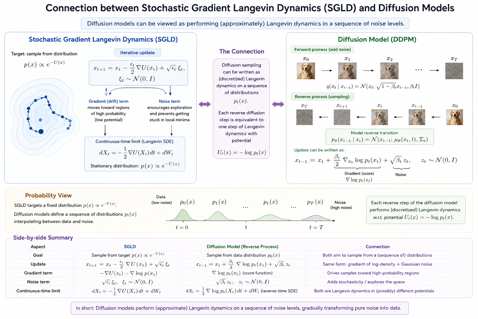
The update rule for SGLD is:
\[x_{t+1} = x_t + \eta \nabla_x \log p(x_t) + \sqrt{2\eta}\,\epsilon_t, \qquad \epsilon_t \sim \mathcal{N}(0, I)\]where:
-
\(\eta\) is the step size,
-
\(\nabla_x \log p(x_t)\) is the score function, i.e., the gradient of the log-density,
-
\(\epsilon_t\) is Gaussian noise.
The gradient term drives samples toward high-density regions of the target distribution, while the stochastic noise term ensures continued exploration.
This framework is strongly connected to diffusion models. In diffusion modeling:
-
The forward process progressively perturbs data with Gaussian noise until the distribution approaches isotropic Gaussian noise.
-
The reverse process learns to invert this corruption procedure step-by-step.
The reverse diffusion update can be interpreted as a form of Langevin dynamics: \(x_{t-1} \approx x_t + \text{score term} + \text{noise}\)
where the neural network estimates the score function: \(\nabla_x \log p_t(x)\)
for the noisy data distribution at timestep \(t\).
In other words, diffusion models learn how to iteratively move noisy samples toward regions of higher data probability, similar to the mechanism used in SGLD. The denoising network effectively approximates the gradient field of the data distribution across multiple noise scales.
This relationship becomes especially clear in score-based generative models, where training explicitly estimates the score function of progressively noisier distributions. Sampling is then performed using Langevin-style dynamics that gradually refine noise into structured data.
A key distinction is that classical SGLD operates directly on a single target distribution, whereas diffusion models define a sequence of intermediate noisy distributions:\(p(x_0) \rightarrow p(x_1) \rightarrow \dots \rightarrow p(x_T)\)
The model learns reverse transitions between these distributions, making sampling more stable and effective in high-dimensional spaces such as images.
This connection to SGLD is significant because it grounds diffusion models in established principles from statistical mechanics, stochastic processes, and Bayesian sampling theory. It also explains why diffusion sampling behaves as a gradual stochastic refinement process rather than direct deterministic generation.
The Reverse Process: Learning to Denoise
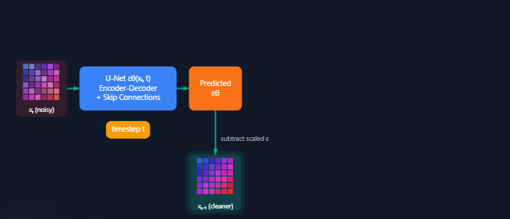
The goal of the reverse diffusion process is to invert the forward noising procedure. Starting from pure Gaussian noise, \(x_T \sim \mathcal{N}(0, I)\), the model progressively removes noise to reconstruct a clean sample \(x_0\). Rather than generating the clean image directly, the network is trained to estimate the noise component present at each timestep. At a given diffusion step \(t\), the model receives the noisy sample and timestep pair \((x_t,t)\), and predicts \(\epsilon_{\theta}(x_t,t)\), where \(\epsilon_{\theta}\) represents the neural network parameterized by \(\theta\).
Intuition
Given this partially corrupted image at timestep \(t\), what noise was added to it?
By accurately estimating the noise, the model can subtract it step by step, gradually transforming random noise into a coherent and realistic sample.
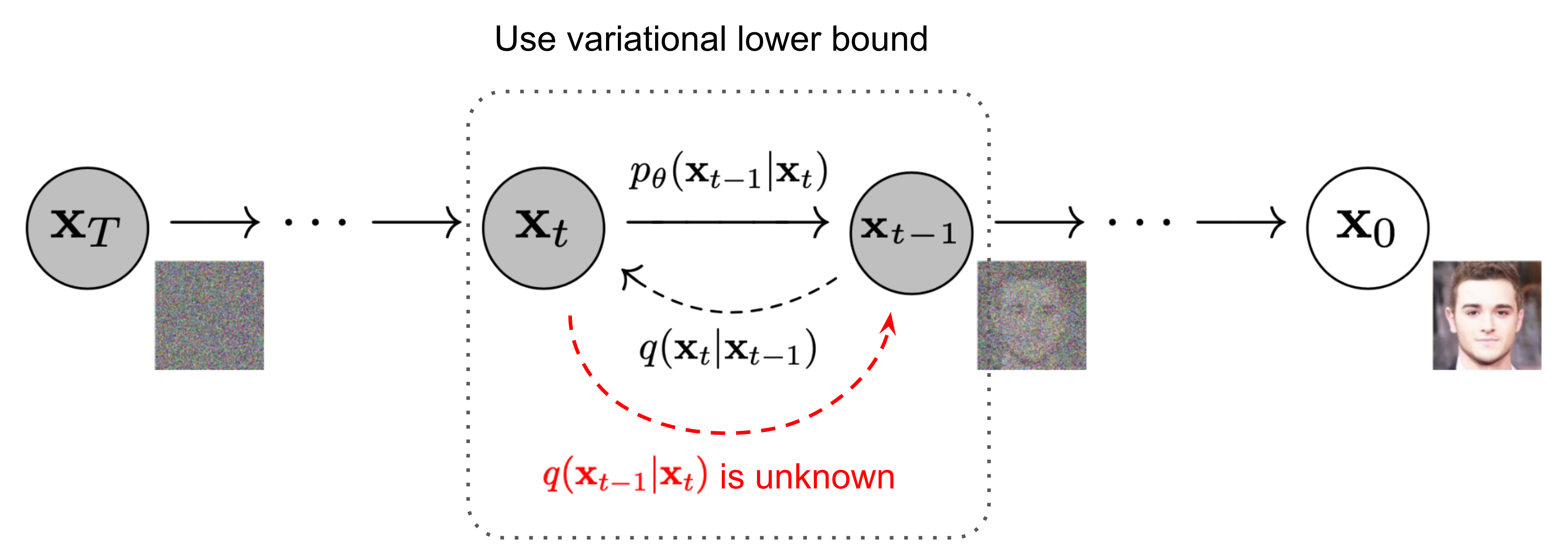
If we could exactly model the reverse transition probabilities \(q(x_{t-1}\mid x_t)\), then we could generate realistic data samples simply by starting from Gaussian noise and repeatedly applying the reverse denoising steps. In other words, diffusion models transform random noise into structured data by learning how to reverse the corruption process.
When the diffusion step size is sufficiently small, the reverse conditional distribution is approximately Gaussian. However, directly computing \(q(x_{t-1}\mid x_t)\) is intractable because it depends on the unknown distribution of all clean images that could have produced the noisy sample \(x_t\). Estimating this distribution would require integrating over the entire data distribution, which is computationally infeasible.
To address this, diffusion models learn a parameterized approximation \(p_\theta(x_{t-1}\mid x_t)\) using a neural network.
Reverse Conditional Distribution
Although the unconditional reverse process is difficult to compute, the reverse conditional becomes tractable if we additionally condition on the original clean image \(x_0\):
\[q(x_{t-1}\mid x_t,x_0) = \mathcal{N} \left( x_{t-1}; \tilde{\mu}_t(x_t,x_0), \tilde{\beta}_t I \right)\]where the posterior variance is
\[\tilde{\beta}_t = \frac{1-\bar{\alpha}_{t-1}} {1-\bar{\alpha}_t}\beta_t\]This result follows from Bayes’ rule and the Gaussian structure of the forward diffusion process. Since both the forward transitions and the accumulated noise process are Gaussian, the posterior distribution also remains Gaussian, allowing the mean and variance to be derived analytically.
Using the forward-process reparameterization, \(x_t = \sqrt{\bar{\alpha}_t}x_0 + \sqrt{1-\bar{\alpha}_t}\,\epsilon, \epsilon\sim\mathcal{N}(0,I)\) the posterior mean can be rewritten entirely in terms of \(x_t\), \(x_0\), and the diffusion coefficients.
Reparameterization Trick
- Direct sampling is a stochastic (random) operation, e.g., \(z \sim \mathcal{N}(\mu,\sigma^2) \). Since the sampled value depends on randomness, the sampling step is non-differentiable, making it difficult to compute gradients and optimize the model using backpropagation.
- To make the model trainable, the reparameterization trick separates randomness from the learnable parameters. Instead of sampling \(z \) directly, we sample noise \( \epsilon \sim \mathcal{N}(0,1) \) and express the sample as \( z=\mu+\sigma\epsilon \).
- This makes the operation differentiable because the randomness is now fixed inside \( \epsilon \), while \( z \) becomes a deterministic mathematical function of \( \mu \) and \( \sigma \). Once \( \epsilon \) is sampled, the computation consists only of multiplication and addition, both of which are differentiable operations.
- As a result, gradients can be computed analytically: \( \frac{\partial z}{\partial \mu}=1, \quad \frac{\partial z}{\partial \sigma}=\epsilon \). Since these derivatives exist, gradients can flow through \( \mu \) and \( \sigma \), making the computation tractable and enabling backpropagation.
- In essence, the reparameterization trick preserves the stochastic nature of sampling while transforming it into a differentiable computation graph, allowing probabilistic models such as VAEs to be trained efficiently using standard gradient descent.
Learning the Reverse Process
During generation, the clean image \(x_0\) is unknown, so diffusion models approximate the reverse conditional using a neural network:
\[p_\theta(x_{t-1}\mid x_t) = \mathcal{N} \left( x_{t-1}; \mu_\theta(x_t,t), \sigma_t^2 I \right)\]where:
-
\(\mu_\theta(x_t,t)\) is the learned reverse-process mean,
-
\(\sigma_t^2\) is either fixed or learned,
-
\(\theta\) denotes the neural network parameters.
Rather than directly predicting the reverse mean, most implementations train the model to predict the added noise \(\epsilon\). This is known as the \(\epsilon\)-prediction formulation.
There are three common ways to parameterize what the network predicts:
\(\epsilon\) -prediction (original DDPM): predict the noise that was added. The denoising update rule then uses this to compute \(x_{t-1}\)
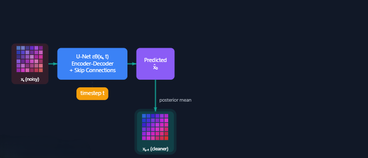
\(x_0\) -prediction: predict the clean image directly. The posterior mean formula then combines this with \(x_t\) to find \(x_{t-1}\)
v-prediction (from progressive distillation): predict a velocity \(v=\sqrt{\bar{\alpha}_t}\epsilon - \sqrt{1-\bar{\alpha}_t}x_0\), which is numerically more stable at both very low and very high noise levels.
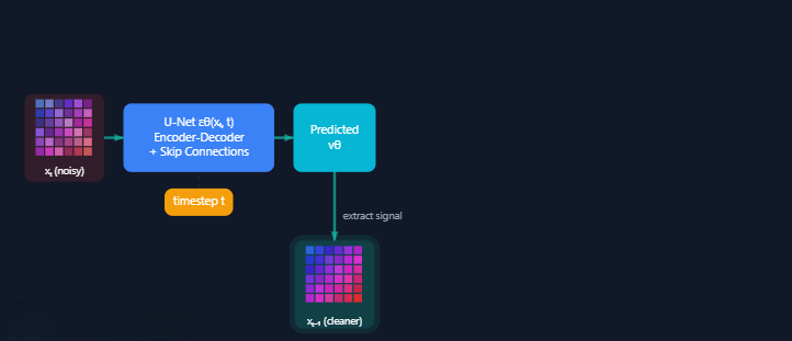
All three parameterizations are mathematically equivalent but have different numerical properties during training.
The reverse mean can then be expressed as:
\[\mu_\theta(x_t,t) = \frac{1}{\sqrt{\alpha_t}} \left( x_t - \frac{\beta_t} {\sqrt{1-\bar{\alpha}_t}} \epsilon_\theta(x_t,t) \right)\]This formulation produces stable optimization behavior because the network learns a well-scaled Gaussian regression task across all timesteps.
The final objective function \(L_t\) then looks as follows (for a random time step \(t\) given \(\epsilon \sim \mathcal{N}(0,1)\)):
\[\mathcal{L} = \left\| \epsilon - \epsilon_\theta(x_t, t) \right\|^2 = \left\| \epsilon - \epsilon_\theta\left( \sqrt{\bar{\alpha}_t}\,x_0 + \sqrt{1-\bar{\alpha}_t}\,\epsilon, t \right) \right\|^2\]Here, \(x_0\) is the initial (real, uncorrupted) image, and we see the direct noise level \(t\) sample given by the fixed forward process. \(\epsilon\) is the pure noise sampled at time step \(t\), and \(\epsilon_\theta(x_t,t)\) is our neural network. The neural network is optimized using a simple mean squared error (MSE) between the true and the predicted Gaussian noise.
For readers interested in the full mathematical derivation of the reverse process, there are several excellent resources available. In particular, Lilan Wang provides a highly accessible explanation in her blog post, and Appendix A of the original 2020 diffusion paper contains a detailed derivation of the underlying equations.
Variational Learning Objective
The overall diffusion framework is closely related to Variational Autoencoders (VAEs). Since the reverse process is probabilistic and latent-variable based, the model can be trained by maximizing a variational lower bound (ELBO) on the data likelihood.
The training objective minimizes the negative log-likelihood:
\[-\log p_\theta(x_0)\]which can be rewritten using variational inference into a tractable objective composed of KL-divergence terms.
The resulting ELBO decomposes into several components:
\[L = L_0 + \sum_{t=1}^{T-1} L_t + L_T\]where:
-
\(L_t\) terms are KL divergences between the true reverse posterior and the learned reverse process,
-
\(L_0\) measures reconstruction quality,
-
\(L_T\) regularizes the final latent distribution toward a standard Gaussian prior.
Most KL-divergence terms compare Gaussian distributions, which means they can be computed analytically in closed form. Additionally, some terms remain constant because they contain no learnable parameters and therefore can be ignored during optimization.
Ho et al. (2020) further simplified this objective and showed that minimizing the variational bound is closely connected to simple noise-prediction losses, which led to the practical diffusion training objective widely used today:
\[\mathbb{E}_{x_0,\epsilon,t} \left[ \| \epsilon - \epsilon_\theta(x_t,t) \|^2 \right]\]This simplified denoising objective became one of the key reasons diffusion models are stable and scalable for high-quality image generation.
Reverse Diffusion via VAEs
The reverse diffusion process can be understood intuitively by comparing diffusion models with Variational Autoencoders (VAEs). Both are latent-variable generative models that learn how to transform simple probability distributions into complex data distributions such as images.
In a VAE, the generative process begins by sampling a latent vector \(z \sim \mathcal{N}(0, I)\) from a simple Gaussian prior. A decoder network then transforms this latent representation into a realistic image:
\[x = \text{Decoder}(z)\]The central idea is that the VAE compresses the data distribution into a lower-dimensional latent space and learns to reconstruct images from those latent variables.
Diffusion models follow a similar philosophy, but instead of relying on a single latent vector \(z\), they use an entire sequence of latent variables: \(x_T \rightarrow x_{T-1} \rightarrow \cdots \rightarrow x_1 \rightarrow x_0\)
where:
-
\(x_T\) is pure Gaussian noise,
-
each intermediate \(x_t\) is a partially denoised representation,
-
\(x_0\) is the final generated image.
Thus, diffusion models can be viewed as performing generation through many small decoding steps rather than one large decoding operation.
Forward Process as the Encoder
The forward diffusion process behaves similarly to the encoder in a VAE.
In a VAE, the encoder learns: \(q_\phi(z \mid x)\) which maps a clean image into a latent Gaussian representation.
Similarly, in diffusion models, the forward process gradually transforms an image into Gaussian noise through repeated applications of: \(q(x_t \mid x_{t-1})\) After many diffusion steps, the final latent state becomes: \(x_T \sim \mathcal{N}(0, I)\) meaning that the original image distribution has been converted into a simple Gaussian prior, analogous to the latent space of a VAE.
The key difference is that VAEs compress information in a single step, while diffusion models corrupt information progressively through many small Gaussian perturbations.
Reverse Process as the Decoder
The reverse diffusion process acts like the decoder of a VAE.
A VAE decoder learns:
\[p_\theta(x \mid z)\]which reconstructs an image from a latent vector.
Similarly, diffusion models learn:
\[p_\theta(x_{t-1} \mid x_t)\]which reconstructs a slightly cleaner image from a noisier one.
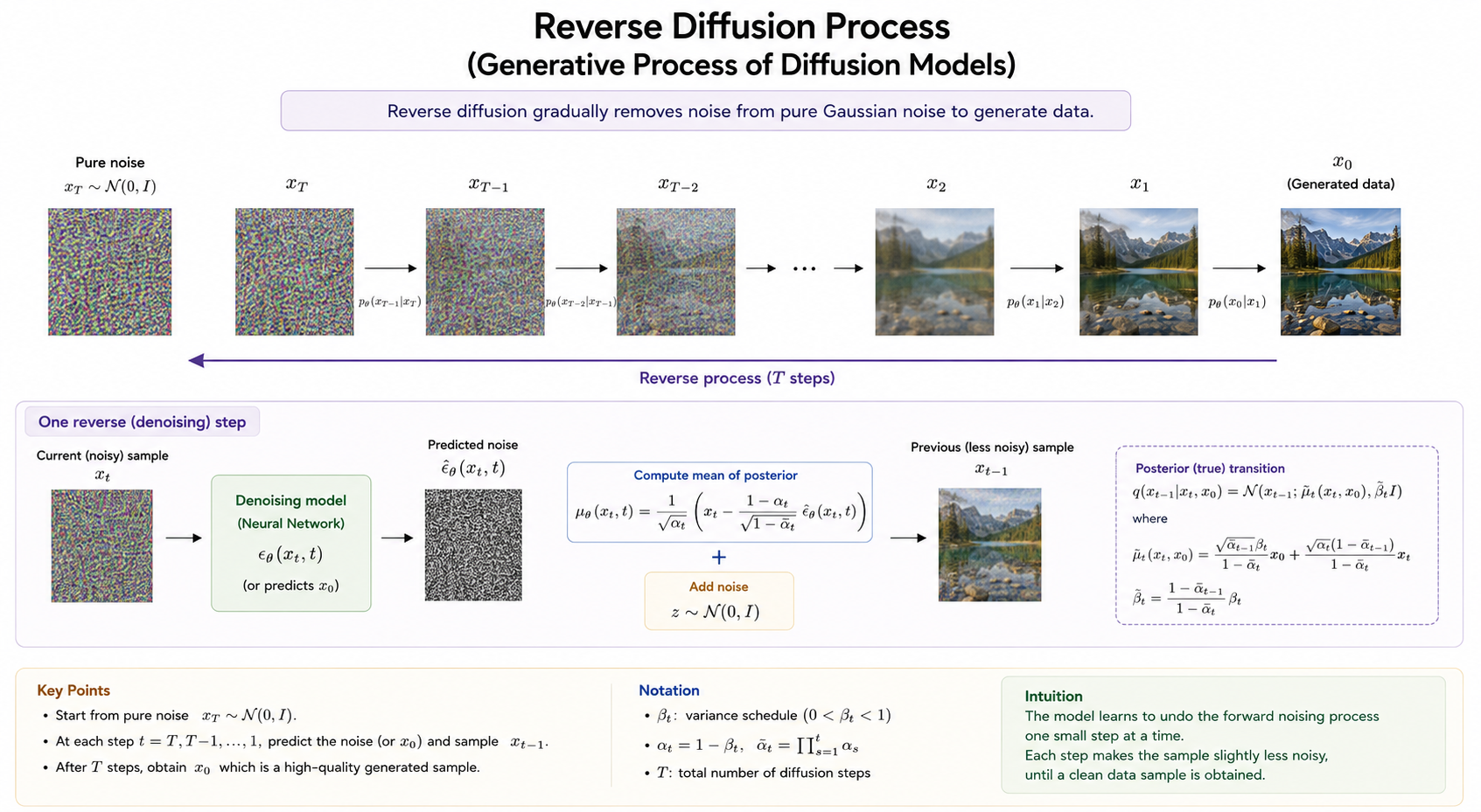
Instead of generating the image in a single step, the diffusion model repeatedly performs small denoising operations:
-
Start with random Gaussian noise \(x_T\),
-
Predict and remove a small amount of noise,
-
Produce a cleaner sample \(x_{t-1}\),
-
Repeat until reaching \(x_0\).
This process can be interpreted as iterative refinement. Each reverse step gradually restores image structure:
-
early steps recover coarse global structure,
-
intermediate steps form semantic shapes,
-
later steps restore fine textures and details.
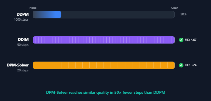
The major drawback is speed: DDPM requires all \(T=1000\) sequential denoising steps. This makes generation roughly \(1000\) times slower than a GAN or VAE, which produce samples in a single forward pass. Two key follow-up works addressed this:
DDIM showed that the reverse process can be reformulated as solving an ordinary differential equation (ODE). This allows deterministic sampling and — crucially — enables skipping timesteps. With only 50 steps, DDIM achieves quality comparable to 1000-step DDPM.
DPM-Solver applies higher-order numerical ODE solvers (analogous to Runge-Kutta methods) to the diffusion ODE. By using second and third-order solvers, it achieves high-quality samples in as few as 10–20 steps — a 50–100x speedup over the original DDPM.
Why the Reverse Process Works
The forward process destroys information gradually using Gaussian noise. Since each corruption step is small and mathematically tractable, the reverse process can also be approximated as a Gaussian transition.
Conditioned on the clean image \(x_0\), the reverse posterior: \(q(x_{t-1} \mid x_t, x_0)\) has a closed-form Gaussian distribution. This is the key insight that makes diffusion models trainable.
The neural network learns to approximate this optimal denoising direction without directly observing the true reverse distribution during generation.
Intuition
Effectively, the model learns: Given a noisy image at timestep \(t\), what noise component was likely added?
Once the predicted noise is removed, the sample moves slightly closer to the clean data manifold.
Relationship to the ELBO in VAEs
The connection between diffusion models and VAEs becomes even clearer through the training objective.
VAEs maximize a variational lower bound (ELBO): \(\log p(x) \geq \mathcal{E}_{q(z|x)}[\log p(x|z)] - D_{KL}(q(z|x)\|p(z))\) Diffusion models derive a closely related variational objective, except the latent variables now correspond to the entire diffusion trajectory: \(x_1, x_2, \dots, x_T\) The diffusion ELBO decomposes into KL-divergence terms between:
-
the true reverse diffusion distributions,
-
and the learned reverse process.
Therefore, diffusion models can be interpreted as deep hierarchical VAEs with thousands of latent layers, where each layer performs a very small denoising transformation.
This interpretation helps explain why diffusion models generate high-quality samples:
-
each denoising step is relatively simple,
-
generation proceeds gradually and stably,
-
the model never needs to reconstruct the entire image in one difficult step.
In contrast, VAEs often struggle because a single decoder must reconstruct the full image from one compressed latent vector, which can produce blurry outputs. Diffusion models avoid this bottleneck by distributing the generation process across many incremental refinement steps.
The U-Net Architecture for Noise Prediction
The neural network \(\epsilon_\theta\) in a diffusion model is designed to take a noisy image \(x_t\) and a timestep \(t\) as input, and predict the noise component added during the forward diffusion process. The most widely used architecture for this task is the U-Net, originally introduced by Ronneberger et al. for biomedical image segmentation and later adapted for diffusion models.
The defining characteristic of the U-Net is its encoder-decoder structure with skip connections. The encoder progressively downsamples the input image using strided convolutions or pooling operations, transforming the image into increasingly abstract feature representations. Early layers capture fine local details such as edges and textures, while deeper layers encode higher-level global structure.
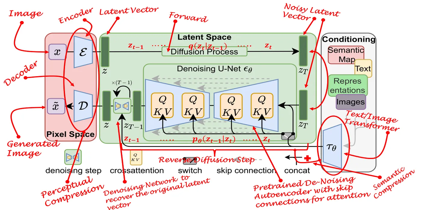
The decoder then progressively upsamples these compressed representations back to the original image resolution using transposed convolutions or interpolation-based upsampling. To preserve spatial detail, skip connections transfer feature maps directly from encoder layers to their corresponding decoder layers. These shortcuts prevent the loss of fine-grained information that would otherwise occur if all image structure had to pass solely through the low-dimensional bottleneck representation.
Diffusion-Specific Adaptations
To function effectively within diffusion models, the standard U-Net is augmented with several important architectural modifications.
Timestep Embeddings
The model must know the current diffusion timestep \(t\), since denoising behavior changes dramatically across the diffusion trajectory. The scalar timestep is therefore converted into a high-dimensional embedding using sinusoidal positional encodings, similar to those used in transformer architectures.
These embeddings are passed through small feed-forward networks and injected into the U-Net at multiple resolution levels. This conditioning allows the network to adapt its behavior depending on the current noise scale.
Residual Blocks
Most modern diffusion U-Nets replace plain convolutional blocks with residual blocks: \(y = F(x) + x\) Residual connections improve gradient propagation during optimization and enable substantially deeper networks without instability. They also help preserve low-level image information throughout the denoising process.
Self-Attention Layers
Self-attention modules are typically inserted at lower spatial resolutions, where feature maps are small enough to make attention computationally affordable.
These layers allow the model to capture long-range spatial dependencies between distant image regions. For example, maintaining globally consistent scene composition—such as coherent lighting, object placement, or semantic relationships between sky, grass, and buildings—requires interactions between pixels that may be far apart spatially.
Attention therefore complements convolutional layers, which are inherently local.
Group Normalization
Diffusion models are often trained with relatively small batch sizes due to the large memory requirements of high-resolution image generation. As a result, batch normalization becomes unstable.
Instead, diffusion U-Nets commonly use group normalization, which normalizes activations across groups of feature channels rather than across batch dimensions. This produces more stable training dynamics under memory-constrained settings.
Multi-Scale Denoising Behavior
A major advantage of the U-Net architecture is that the same network can operate across all diffusion timesteps \(T\). As a result, the model learns different denoising behaviors depending on the current noise level.
-
At high noise levels (early generation stages), the model focuses primarily on recovering coarse global structure and low-frequency information.
-
At low noise levels (later stages), the model refines high-frequency details such as textures, edges, and fine visual patterns.
This naturally creates a coarse-to-fine generation process, where global semantic structure emerges first and detailed appearance is progressively refined over successive denoising steps.
Diffusion Model Algorithm
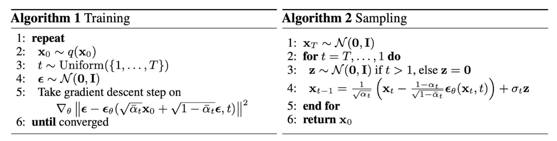
Training
This algorithm teaches the model how to remove noise from images.
Intuition
The model learns by repeatedly seeing corrupted images and figuring out how to clean them.
-
Pick a real image.
-
Choose a random noise level \(t\).
-
Add random Gaussian noise to the image.
-
Give the noisy image to the neural network.
-
The network tries to predict the exact noise added.
-
Compare the prediction with the real noise and update the model using gradient descent.
-
Repeat until the model learns to denoise well.
Sampling / Image Generation
This algorithm generates new images using the trained model.
Intuition
The model starts from static noise and progressively “cleans” it into a meaningful image.
-
Start with pure random noise.
-
Move backward from timestep \(T\) to \(1\).
-
At each step, the model predicts the noise in the image.
-
Remove a small amount of noise.
-
Repeat the process gradually.
-
The random noise slowly turns into a realistic image.
Key Parameters in Diffusion Models
Designing an effective diffusion model requires balancing several important hyperparameters that directly influence generation quality, computational efficiency, and controllability.
Number of Timesteps \((T)\)
The parameter \(T\) determines the number of denoising steps used in the diffusion process.
-
Larger values of \(T\) create a more gradual and fine-grained corruption and denoising trajectory.
-
Smaller values reduce computational cost but may degrade generation quality.
During training, diffusion models are commonly trained with: \(T \in [100,1000]\) At inference time, modern samplers such as DPM-Solver++ can generate high-quality samples using significantly fewer steps, often in the range of 20–50 iterations.
Increasing \(T\) generally improves fidelity and stability, but sampling latency grows proportionally.
Noise Schedule (\(\beta_t\))
The noise schedule controls how rapidly information is destroyed during forward diffusion.
Two commonly used schedules are:
-
Linear schedule
Simple to implement but tends to allocate too many steps to nearly pure noise regions. -
Cosine schedule
Preserves image structure longer and allocates more steps to informative intermediate noise levels, usually resulting in higher-quality outputs.
The schedule strongly affects optimization stability and perceptual quality.
Guidance Scale (\(w\))
The guidance scale controls the strength of conditioning during generation, especially in classifier-free guidance.
-
Higher values of \(w\) increase prompt adherence and semantic consistency.
-
Lower values encourage more diversity and natural variation.
Typical ranges are: \(w \approx 7\text{--}12\) for highly prompt-aligned creative generation, and \(w \approx 1\text{--}3\) for more realistic and diverse outputs.
Very large guidance values can produce oversaturated colors, distorted anatomy, or reduced sample diversity.
Latent Compression Factor
In latent diffusion models such as Stable Diffusion, images are compressed into a lower-dimensional latent representation before diffusion is applied.
A standard configuration uses approximately: \(8\times\) spatial compression.
This substantially reduces memory usage and computational cost while preserving most perceptual structure.
However, there is an important tradeoff:
-
Excessive compression removes fine image detail and texture information.
-
Insufficient compression increases computational requirements dramatically.
The compression factor therefore determines the balance between efficiency and reconstruction fidelity.
U-Net Attention Resolution
Self-attention layers are computationally expensive because their memory and compute cost scale quadratically with spatial resolution.
For this reason, diffusion models usually apply attention only at lower-resolution feature maps inside the U-Net.
Adding attention at higher resolutions improves the model’s ability to capture fine-grained long-range dependencies, but significantly increases GPU memory consumption and runtime.
This becomes especially important for high-resolution generation systems.
VAE Regularization Strength
Latent diffusion models rely on a Variational Autoencoder (VAE) to map images into latent space. During VAE training, a KL-divergence regularization term encourages the latent distribution to approximate a Gaussian prior.
The strength of this regularization critically affects latent-space geometry.
-
Excessive regularization forces the latent representation to collapse toward an overly simple distribution, reducing reconstruction quality.
-
Insufficient regularization allows the latent space to become highly irregular and non-Gaussian, making diffusion dynamics difficult to learn.
An effective latent space must therefore remain both expressive and smoothly navigable by the diffusion process.
Tradeoffs Between Parameters
These hyperparameters interact strongly with one another:
-
Larger \(T\) values improve quality but slow sampling.
-
Stronger guidance improves controllability but reduces diversity.
-
Higher attention resolution improves coherence but increases memory usage.
-
Stronger compression improves efficiency but sacrifices detail.
Modern diffusion systems are largely engineered around carefully balancing these competing objectives to achieve scalable, high-quality generation.
Conclusion
Generative models can be broadly categorized into two main families based on how they learn and generate data distributions:
- Likelihood-Based Models — These models explicitly estimate or optimize the probability distribution of the data. Representative approaches include:
- Autoregressive Models
- Variational Autoencoders (VAEs)
- Normalizing Flows
- Energy-Based Models (EBMs)
- Diffusion Models
- Likelihood-Free Models — These models generate realistic samples without directly modeling data likelihood. The most prominent example is:
- Generative Adversarial Networks (GANs)
Among these approaches, diffusion models have recently emerged as one of the most effective and reliable generative modeling frameworks. Diffusion models offer a powerful alternative to GANs and VAEs by replacing single-step generation with a sequence of small, stable denoising steps. This gradual reverse process mitigates issues such as adversarial instability in GANs and the blurry reconstructions often observed in VAEs. By formulating generation as iterative refinement, diffusion models are able to capture complex multimodal data distributions and synthesize sharp, high-quality samples.
A central component of modern diffusion architectures is the U-Net–based noise predictor, which enables the model to handle varying noise levels while recovering both global structure and fine-grained details. Furthermore, carefully designed noise schedules, such as cosine schedules, improve learning efficiency by allocating modeling capacity to the most informative stages of the denoising process. Techniques including classifier guidance, classifier-free guidance, and latent-space diffusion further enhance controllability, fidelity, and computational efficiency.
Overall, diffusion models have become the dominant paradigm for high-quality image synthesis due to their strong theoretical foundation, training stability, and impressive empirical performance. As research continues, future advancements are expected to significantly reduce sampling time while preserving the robustness, expressiveness, and realism that make diffusion models so successful.
References
-
Dhariwal, Prafulla, and Alexander Nichol. “Diffusion models beat gans on image synthesis.” Advances in neural information processing systems 34 (2021): 8780-8794.
-
Ho, J., Jain, A., & Abbeel, P. (2020). Denoising Diffusion Probabilistic Models. arXiv:2006.11239.
-
Nichol, A., & Dhariwal, P. (2021). Improved Denoising Diffusion Probabilistic Models. arXiv:2102.09672.
-
Sohl-Dickstein, J., Weiss, E. A., Maheswaranathan, N., & Ganguli, S. (2015). Deep Unsupervised Learning using Nonequilibrium Thermodynamics. arXiv:1503.03585.
-
Ho, J., & Salimans, T. (2022). Classifier-Free Diffusion Guidance. arXiv:2207.12598.
-
Weng, L. (2021). What are diffusion models? Lil’Log. Retrieved from https://lilianweng.github.io/posts/2021-07-11-diffusion-models/
-
Ronneberger, O., Fischer, P., & Brox, T. (2015). U-Net: Convolutional Networks for Biomedical Image Segmentation. arXiv:1505.04597.
-
Erdem, K. (2023). Step by Step Visual Introduction to Diffusion Models. Retrieved from https://erdem.pl/2023/11/step-by-step-visual-introduction-to-diffusion-models
-
Ho, Jonathan, Ajay Jain, and Pieter Abbeel. “Denoising diffusion probabilistic models.” Advances in neural information processing systems 33 (2020): 6840-6851.
-
Lu, Cheng, et al. “Dpm-solver: A fast ode solver for diffusion probabilistic model sampling in around 10 steps.” Advances in neural information processing systems 35 (2022): 5775-5787.
Citation
If you found this useful, please cite this as:Patil, Aniket (May 2026). VAE-Inspired Diffusion Revolution. https://AniketP04.github.io.
or as a BibTeX entry:
@article{patil2026vae-inspired-diffusion-revolution,
  title   = {VAE-Inspired Diffusion Revolution},
  author  = {Patil, Aniket},
  year    = {2026},
  month   = {May},
  url     = {https://AniketP04.github.io/blog/2026/VAE-Inspired_Diffusion_Revolution/}
}
Enjoy Reading This Article?
Here are some more articles you might like to read next: