Active and Volumetric Stereo
- Beyond Passive Vision: Active Stereo and Volumetric 3D Reconstruction
- Introduction: The Hardest Part of Stereo Vision
- Part 1: Active Stereo — Illuminating the Correspondence Problem Away
- Part 2: Volumetric Stereo — Turning the Problem Inside Out
- Comparing the Three Volumetric Methods
- Active Stereo vs. Volumetric Stereo: When to Use What
- Conclusion: Rethinking the Problem to Solve It
Beyond Passive Vision: Active Stereo and Volumetric 3D Reconstruction
How computers use structured light, shadows, and volumetric reasoning to reconstruct the shape of objects — without solving the correspondence problem.
Introduction: The Hardest Part of Stereo Vision
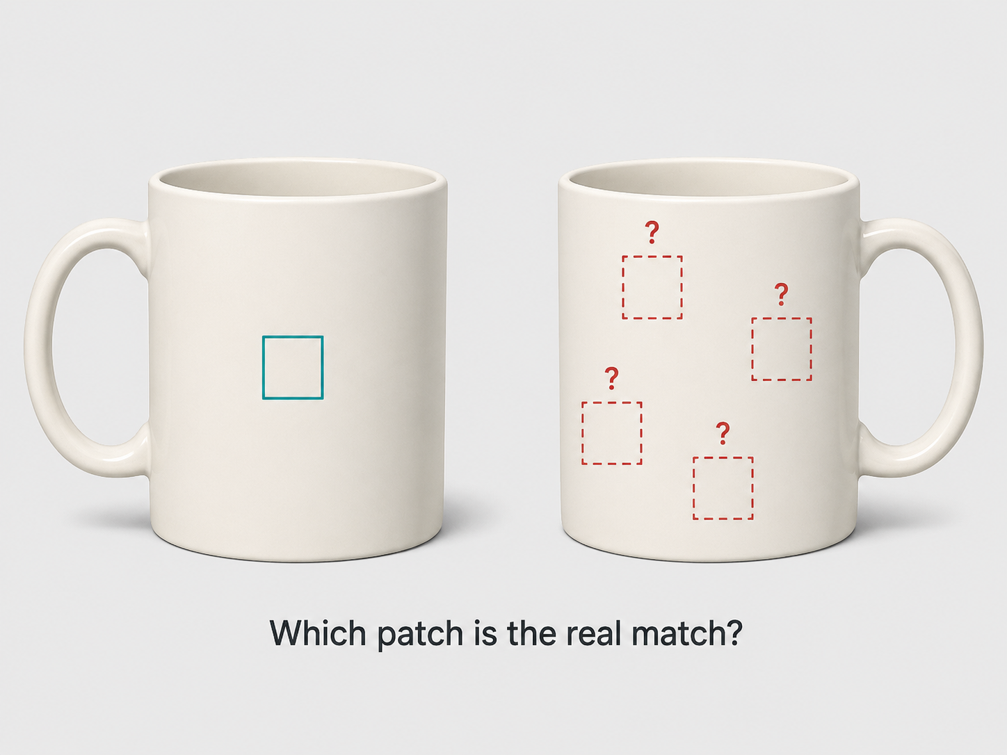
Imagine you are given two photographs of the same coffee mug, taken from slightly different positions. Your task is to figure out the 3D shape of the mug. Conceptually, the approach is clear: find matching points across the two images, then use triangulation to recover each point’s position in 3D space. Easy enough in theory.
But in practice, this task — called the correspondence problem — is notoriously difficult. How do you know whether pixel $(100, 200)$ in the left image actually corresponds to pixel $(98, 197)$ in the right image? On a uniformly white ceramic mug, most pixels look nearly identical. A small patch of the surface could match dozens of other patches. Texture-less regions, reflective surfaces, and repeated patterns all make the correspondence problem ambiguous, and errors in correspondence translate directly into errors in 3D reconstruction.
The methods covered in previous discussions — triangulation, structure from motion, bundle adjustment — all assumed that the correspondence problem had already been solved. But as we push toward practical 3D reconstruction systems, this assumption becomes the main bottleneck.
This article explores two families of techniques that take radically different approaches to circumventing or sidestepping the correspondence problem entirely. Active stereo sidesteps it by projecting known patterns into the scene, making correspondences trivially identifiable. Volumetric stereo inverts the problem altogether, asking not “which pixels correspond?” but rather “which candidate 3D points are geometrically consistent with the images?”
Both approaches have powered real-world applications — from the sub-millimeter digitization of Renaissance masterpieces to the depth sensors embedded in consumer gaming devices — and together they represent a rich toolkit for shape acquisition that complements the passive methods we have discussed so far.
Part 1: Active Stereo — Illuminating the Correspondence Problem Away
The Core Idea
The fundamental insight of active stereo is elegantly simple: if you do not know which parts of the scene correspond across your two cameras, just mark them yourself. Instead of passively relying on the scene’s existing texture, you project a known pattern onto the object and let the pattern carry the correspondence information.
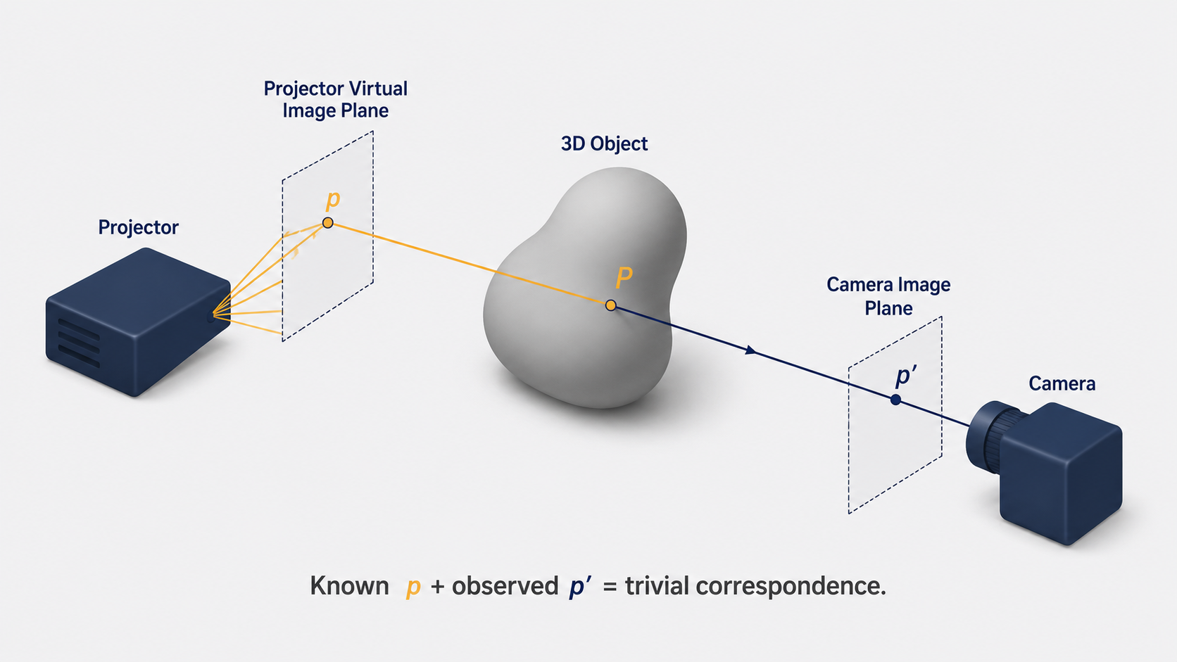
In a standard stereo setup, you have two cameras. Active stereo replaces one camera with a projector — a device that can emit controlled patterns of light (typically a digital light projector, or DLP). The projector-camera pair defines the same epipolar geometry as a camera-camera pair, with the projector’s image plane serving as a “virtual camera” plane. The key difference: while a camera passively records light, the projector emits it with full knowledge of what is being emitted.
Here is the crucial consequence. When the projector sends a ray of light through a specific pixel $p$ in its virtual image plane, that ray illuminates a unique physical point $P$ in the scene. The camera, observing the scene, captures the reflection of that illuminated point at pixel $p’$ in its image. Because you know exactly what the projector sent ($p$ is fully known), identifying $p’$ in the camera image gives you an immediate, unambiguous correspondence. The matching problem reduces to asking: “where in the camera image can I see the pattern I just projected?” — a far easier question than passive feature matching.
From Points to Lines: The Scanning Stripe Approach
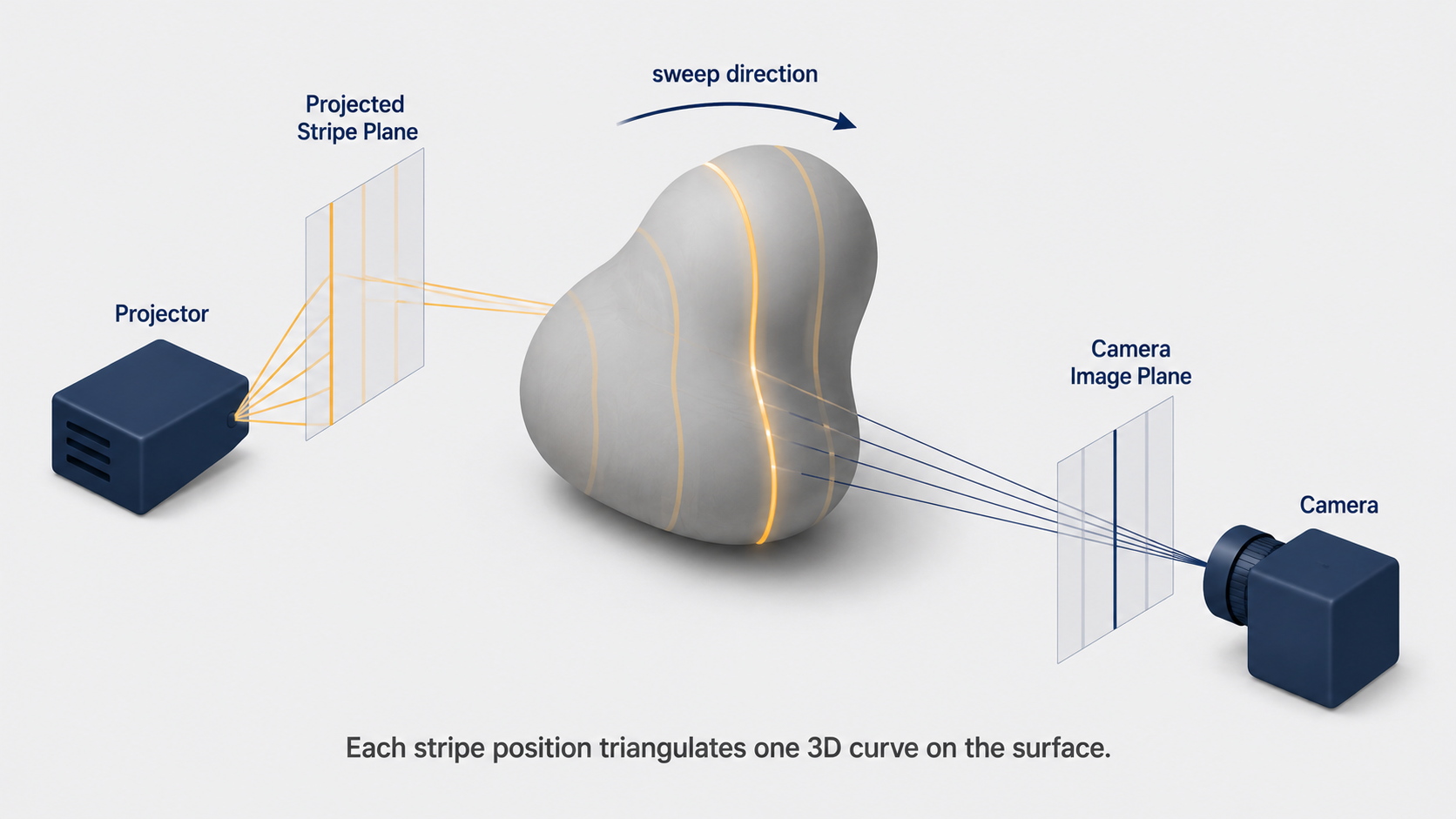
Projecting a single point tells you the 3D location of one surface point. To reconstruct an entire surface, the simplest active stereo strategy is to project a thin vertical stripe (a line of light) across the scene. The stripe illuminates a curve on the object’s surface, which appears as a bright line in the camera image.
If the projector and camera are configured to be rectified (their image rows aligned with the epipolar lines), then the correspondence search collapses to a simple one-dimensional problem: each point on the observed stripe $s’$ in the camera can only correspond to the point on the same horizontal epipolar line in the projector. With correspondences established, every point on the illuminated stripe $S$ is triangulated, recovering a 3D curve on the surface.
By sweeping the stripe laterally across the scene — one stripe position at a time — and repeating the triangulation for each position, the complete visible surface of the object is reconstructed point by point. This is the principle behind laser line scanning, one of the workhorses of industrial metrology and heritage digitization.
The historical pinnacle of this approach came in 2000, when Marc Levoy and his team at Stanford applied a finely calibrated laser scanner to Michelangelo’s Pietà, achieving sub-millimeter accuracy across the entire sculpture. The result was a digital 3D model of extraordinary fidelity — a testament to how powerful active stereo becomes when the system is carefully engineered.
The Calibration of an Active Stereo System
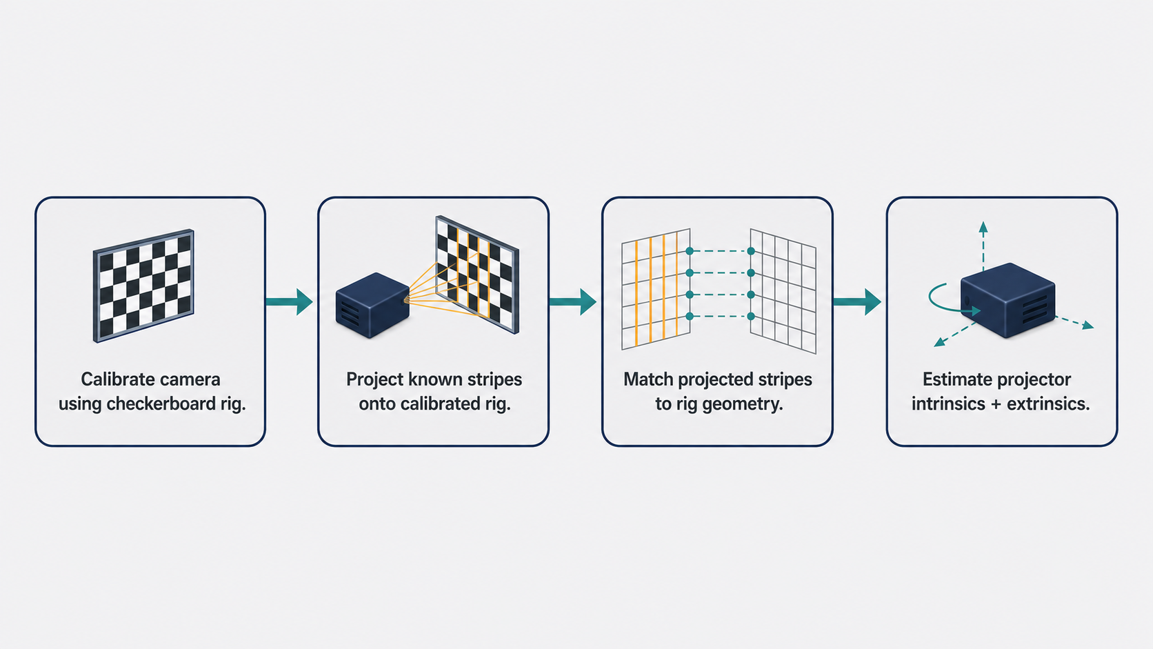
An active stereo system must be calibrated before it can produce accurate measurements. The camera is calibrated first using standard techniques — a checkerboard calibration rig, for instance — to recover its intrinsic parameters and lens distortions. Then, with the camera calibrated, known stripes are projected onto the calibration rig. By observing where these stripes appear in the camera image and matching those observations to the known geometry of the rig, constraints can be established to estimate the projector’s intrinsic and extrinsic parameters (its focal length, principal point, and pose relative to the camera). Once both devices are calibrated, the system is ready to triangulate.
A Cheaper Alternative: Shadow Stripes
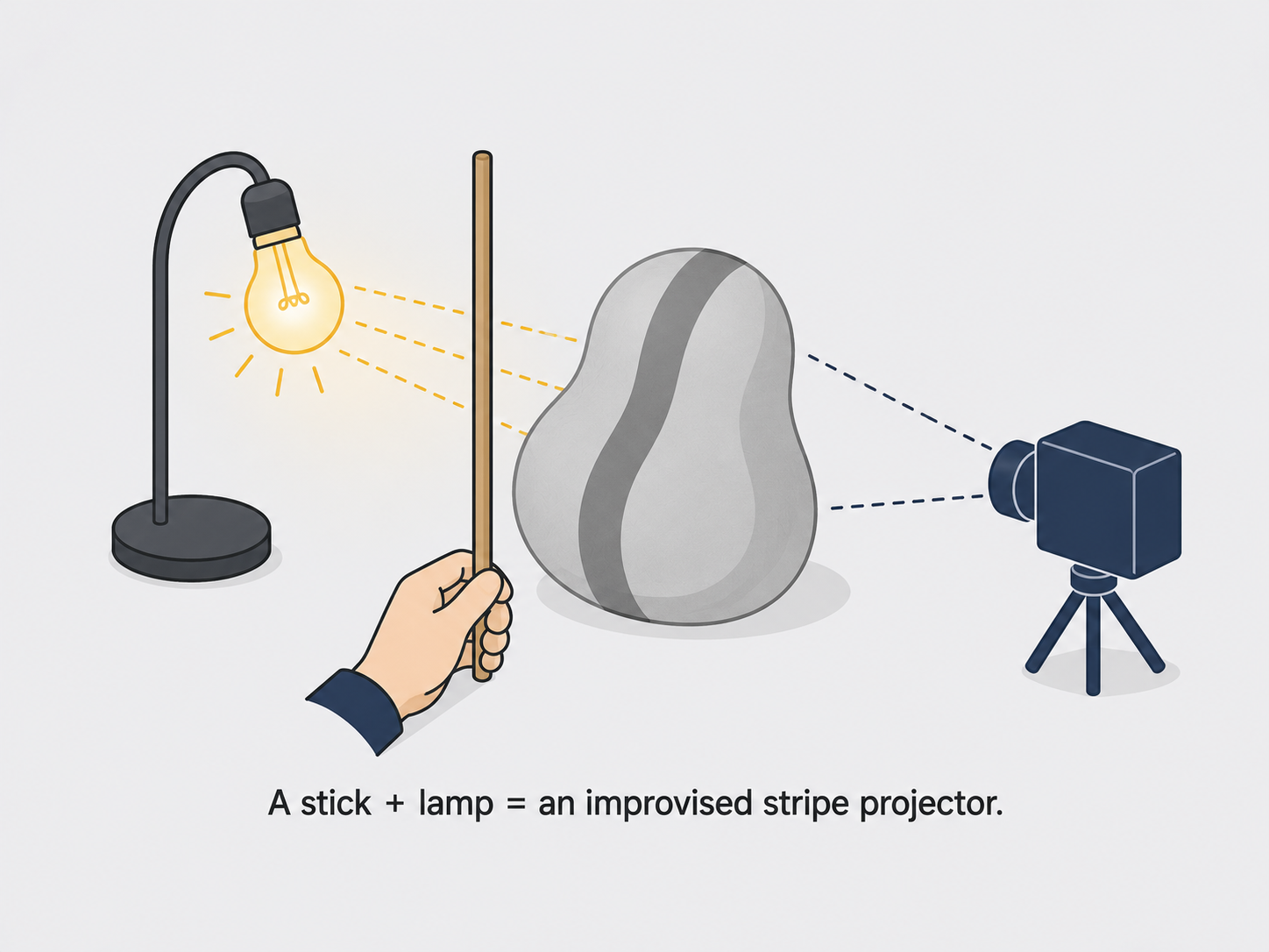
What if you cannot afford a high-quality digital projector? An inexpensive but surprisingly effective alternative uses shadows instead of projected light. Place a thin stick between the object and a known light source. The stick’s shadow creates a dark stripe on the object’s surface — functionally equivalent to a projected stripe, but achieved with nothing more than a stick and a lamp.
Moving the stick progressively casts different shadow stripes across the object, and the reconstruction proceeds exactly as in the scanning stripe approach. The method is cheap and requires no specialized equipment beyond a camera, a light source, and a stick. The trade-off is accuracy: the sharpness and position of a shadow stripe is more sensitive to the geometry of the stick, the light source, and the camera, making calibration more demanding and reconstruction less precise.
Single-Shot Reconstruction: Structured Light
The scanning stripe method has a significant practical limitation: it requires the object to be completely still while the stripe sweeps across it. Any motion during the scan produces artifacts. For dynamic scenes — a person moving, a robot manipulating an object, a face making expressions — scanning is far too slow.
The solution is structured light: rather than scanning one stripe at a time, project an entire pattern of multiple distinctively-colored or distinctively-coded stripes simultaneously, illuminating the entire visible surface in a single exposure. If the stripe pattern is designed such that every stripe has a unique color (or unique local code), then the camera can identify which stripe is which from a single image, and all correspondences are established at once.
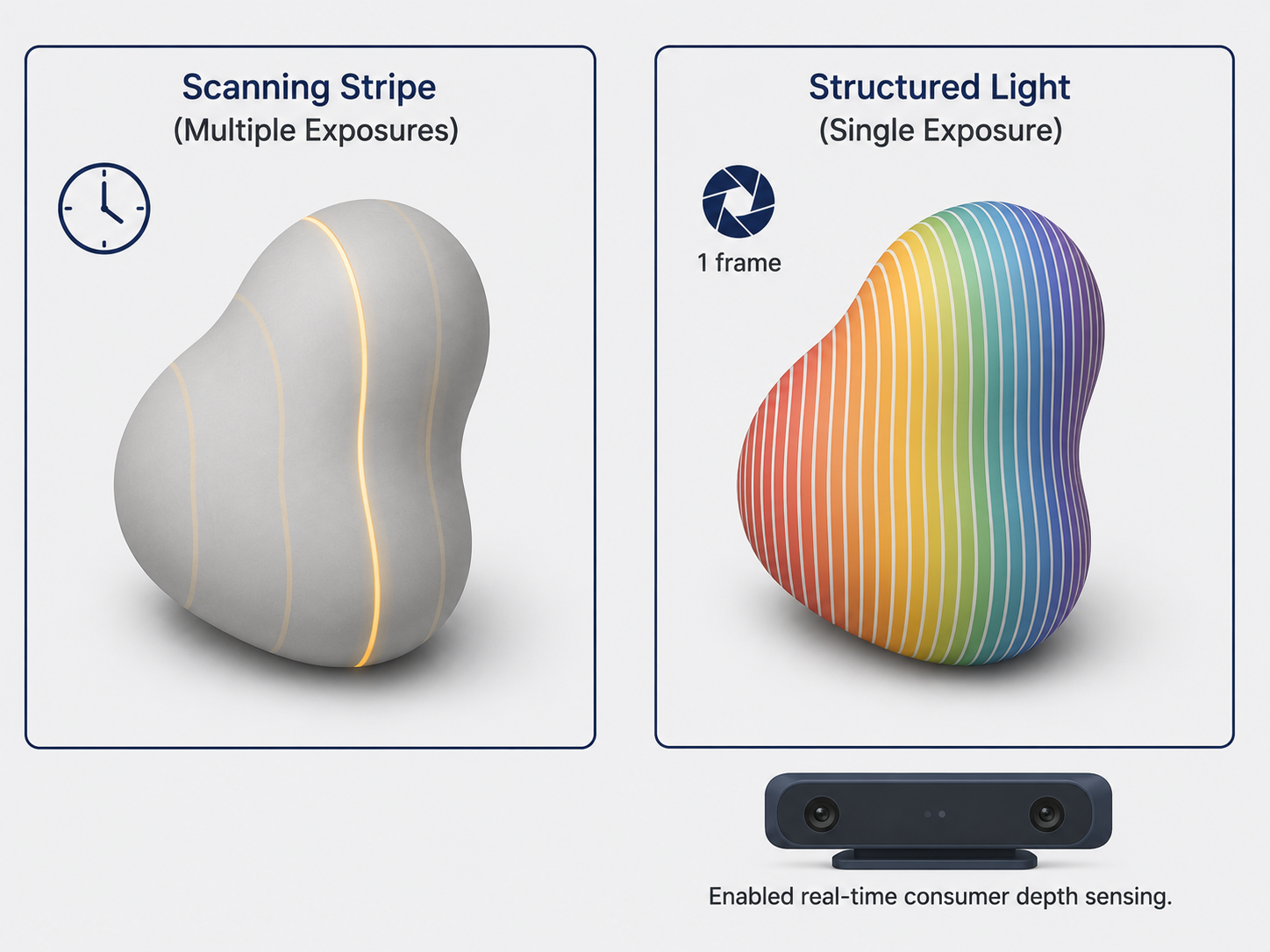
Figure 3 in the source notes illustrates this: a pattern of differently-colored vertical stripes is projected onto an object, and the camera observes the distorted, color-coded pattern on the surface. By identifying each stripe’s color, correspondences are established across the entire surface simultaneously, and the full 3D shape is recovered from a single projected frame.
This idea powered an iconic consumer product: the original Microsoft Kinect. Rather than visible colored stripes (which would be disturbing in normal use), Kinect used an infrared laser projector to project a pseudo-random dot pattern invisible to the human eye. An infrared camera captured the pattern as it deformed over the scene’s geometry. By matching the deformed pattern back to the known projected pattern, per-pixel depth estimates were computed in real time at video frame rates — enabling body tracking, gesture interfaces, and countless downstream applications.
Part 2: Volumetric Stereo — Turning the Problem Inside Out
A Completely Different Philosophy
Active stereo still relies on a projector-camera geometry that fundamentally resembles traditional stereo — it just makes correspondences easy. Volumetric stereo takes a much more radical departure. Rather than finding correspondences and triangulating forward, it starts with candidate 3D points and asks whether they are consistent with what the cameras observe.
Here is the mental model. Imagine you know that the object you want to reconstruct is sitting inside a glass box — a bounded working volume. Fill that box with a dense 3D grid of tiny cubes called voxels (short for volumetric pixels). Each voxel is a candidate piece of the object. Your task is to figure out which voxels are actually occupied by the object and which are empty space.
For each candidate voxel, project it into all the calibrated cameras and check: does what the cameras see at those projection locations agree with what you would expect if that voxel were part of the object? If yes, keep the voxel. If no, discard it. The surviving voxels, after checking all candidates, form your 3D reconstruction.
This approach elegantly sidesteps the correspondence problem. You never ask “which pixel in image 1 matches which pixel in image 2?” Instead, you ask “is this specific 3D location consistent with all available views?” The consistency check is local to each candidate voxel.
Of course, everything hinges on how you define “consistent.” Different choices lead to different algorithms. We will examine three: space carving, shadow carving, and voxel coloring.
Method 1: Space Carving — Using Silhouettes as Constraints
The Geometric Insight
Space carving begins with a beautiful geometric observation: the silhouette of an object — the boundary of its projection in an image — is a powerful constraint on its 3D shape.
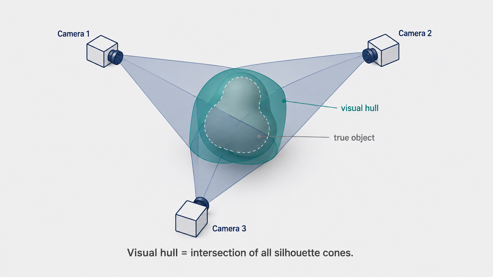
Think about what a silhouette tells you. When you photograph a ball against a white background, the silhouette is a circle. Every 3D point that could possibly produce that circular silhouette must lie inside the visual cone — the cone-shaped region formed by shooting rays from the camera center through every pixel on the silhouette boundary. Any 3D point outside this cone would project outside the silhouette, so it cannot belong to the object.
Now here is the power of multiple views. From camera 1, you compute a visual cone. From camera 2, you compute a different visual cone. Since the object must be inside both cones simultaneously, it must lie in their intersection. Add a third camera, and the object must be in the intersection of three cones. More cameras tighten the estimate.
The intersection of all visual cones from all cameras is called the visual hull. The visual hull is always a conservative upper bound on the object’s shape — the real object fits inside it, but the visual hull may contain regions that are not part of the object. You can think of it as the most the silhouettes can tell you without any other information.
Practical Implementation: Voxels and Projection
In practice, space carving is implemented on a discrete voxel grid:
- Initialize the working volume as a full voxel grid, where every voxel is initially marked as “occupied.”
- For each camera, extract the silhouette of the object in that image. If the background is controlled — for example, using a green screen — this segmentation is straightforward.
- For each voxel, project it into the camera image.
- If the voxel’s projection falls outside the silhouette, the voxel cannot be part of the object — remove it (carve it away).
- After processing all cameras, the remaining voxels form the visual hull estimate.
The name “space carving” evokes the right mental image: you start with a solid block and progressively chisel away voxels that are inconsistent with each silhouette view, like a sculptor revealing the form hidden inside a block of marble.
An important property of the algorithm is that it is conservative: it never removes a voxel that might genuinely be part of the object (assuming perfect silhouettes). Every removal is justified by the certainty that the voxel falls outside the object’s projection in at least one view. This means the reconstruction always contains the true object — but may contain extra material around it.
Limitations of Space Carving
Space carving is elegant and avoids the correspondence problem entirely, but it has real limitations.
The first is computational cost. The algorithm iterates over every voxel in the grid and projects it into every camera. If you halve the voxel size to double the reconstruction resolution, the number of voxels increases by a factor of $2^3 = 8$ in 3D — a cubic relationship. Fine reconstructions require enormous grids and corresponding computation time. Hierarchical data structures like octrees, which adaptively refine the voxel grid only where needed, can mitigate this.
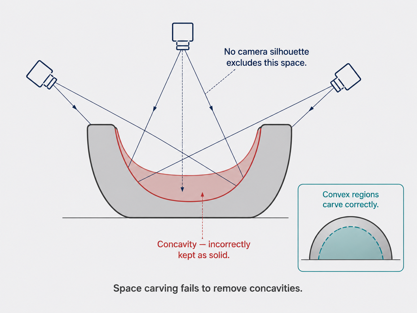
The second limitation is concavities. Space carving fundamentally cannot reconstruct concave regions of an object’s surface. Why? Consider a bowl viewed from above. The inside of the bowl is a concavity — a region scooped inward. But from any camera that can see the bowl, the silhouette includes the entire bowl including its rim. The visual hull therefore fills in the interior of the bowl, treating it as solid. Carving cannot reach into the concavity without removing material that genuinely belongs to the object.
To see this more precisely: a voxel inside a concavity projects within the silhouette in every view, so space carving keeps it — incorrectly. The algorithm has no way to know the concavity exists based on silhouettes alone. The only concavities that space carving handles correctly are holes through the object (like a donut), where the hole is visible in the silhouette from certain angles.
Method 2: Shadow Carving — Illuminating Concavities
Shadow carving addresses the concavity limitation by introducing an additional source of information: self-shadows.
When an object with a concave region is illuminated from the side, its protruding parts often cast shadows onto the concave area itself. The shape and extent of these self-shadows carry geometric information about the concavity that the silhouette alone cannot provide.
The Setup
The shadow carving setup augments the space carving system with a carefully arranged array of lights at known positions surrounding the camera. The object is placed on a turntable so it can be observed from multiple angles. By turning individual lights on and off in sequence, the object is illuminated from different directions, producing different self-shadow patterns on its surface for each lighting configuration.
The Algorithm
Shadow carving begins by running space carving with the silhouette, producing an initial visual hull that over-estimates the object’s volume. The subsequent shadow carving steps then refine this hull by carving away voxels in concave regions.
For each light source and each camera view, the algorithm identifies the shadow cast by the object in the camera image. This shadow, like the silhouette, defines a visual cone — the “shadow cone” — emanating from the light source through the shadow boundary in the image. The key logical step is subtle but powerful: a voxel that falls inside both the shadow cone of the light source and the visual cone of the camera simultaneously cannot be part of the object. If it were, it would be both visible to the camera (the camera’s visual cone implies it is in the camera’s line of sight within the silhouette) and in shadow (the light’s shadow cone implies it is occluded from the light). The presence of a shadow on the object’s surface implies that something is between the light and the shadowed region — and those “something” voxels can be refined away from the concavity.
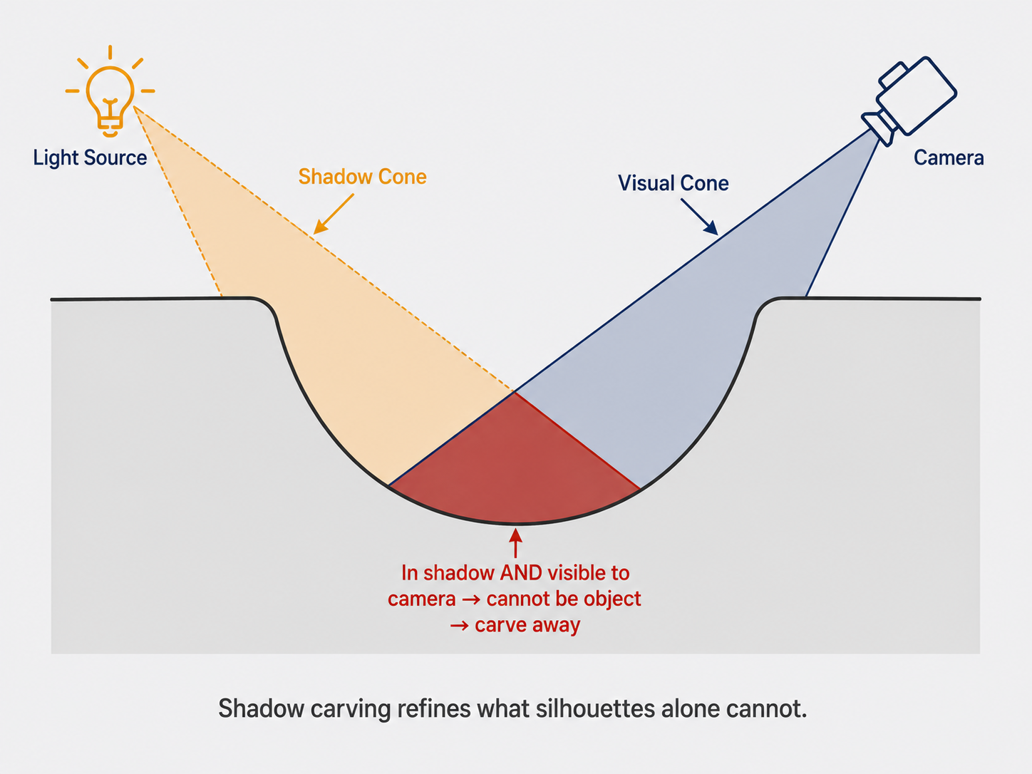
By cycling through all lights and all views, shadow carving progressively carves away voxels in concave regions that space carving would have left untouched, producing a tighter estimate of the true object shape.
Trade-offs
Shadow carving shares the cubic scaling of space carving. With $N$ lights, each voxel must be projected into the camera and into each of the $N$ light sources — multiplying the computation by approximately $N + 1$ relative to vanilla space carving.
The method also has material restrictions. It fundamentally relies on detecting sharp, clear shadows in the camera image. Objects with highly reflective surfaces scatter light in complex ways that smear shadow boundaries, making detection unreliable. Similarly, very dark (low-albedo) objects absorb most incident light and produce faint shadows that are difficult to detect against a dark object surface. For such materials, shadow carving degrades significantly.
Method 3: Voxel Coloring — Consistency Through Color
The third volumetric stereo technique, voxel coloring, replaces the geometric consistency check of space carving (silhouette containment) with a photometric one: color consistency.
The Core Idea
The idea is intuitive. If a voxel truly lies on the surface of an object, then projecting that voxel into multiple cameras should yield similar colors in all of them — because they are all looking at the same physical surface point. If the colors are wildly different across views, the voxel is probably not on the surface (perhaps it is in empty space, where different cameras see different background colors projected back to that location).
For each voxel in the working volume, voxel coloring:
- Projects the voxel into every camera that has a clear line of sight to it.
- Samples the image color at each projection location.
- If the sampled colors are mutually consistent (within some threshold), marks the voxel as occupied and assigns it the average color.
- If the colors are inconsistent, discards the voxel.
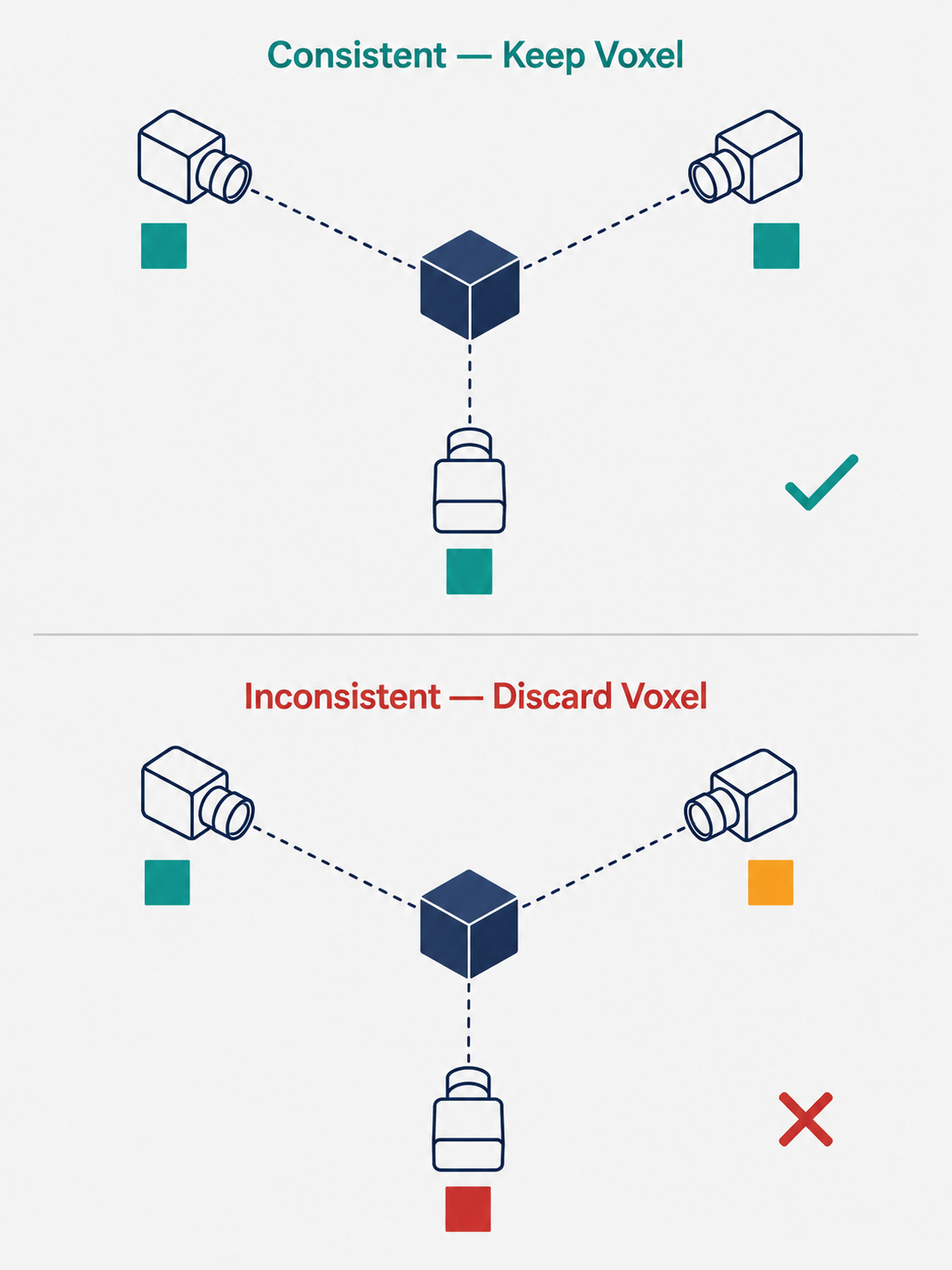
The bonus beyond space carving: the voxels not only capture the object’s shape but also its appearance. The resulting reconstruction is a colored voxel model — simultaneously a geometric and a photometric representation. This makes voxel coloring attractive for applications where texture matters, like cultural heritage digitization or product visualization.
The Lambertian Assumption
Voxel coloring rests on a critical assumption: the object must be Lambertian. A Lambertian surface is one that scatters incoming light uniformly in all directions — a matte surface, like unvarnished wood, rough plaster, or matte paint. The perceived brightness and color of a Lambertian surface is independent of the viewing direction, which is exactly what the color consistency check requires: the same surface point should look the same from camera 1 as from camera 2.
Highly specular (shiny) or reflective objects violate this assumption badly. A polished metal sphere looks different depending on the viewing angle — it reflects the environment, showing different colors to different cameras even though the sphere’s surface material has not changed. For such objects, the color consistency check fails even on voxels that genuinely belong to the object, causing them to be incorrectly discarded.
This is a fundamental physical limitation of photometric consistency methods, not a flaw that can be engineered away without more sophisticated models of surface reflectance.
The Ambiguity Problem and the Visibility Ordering Fix
Vanilla voxel coloring has a subtle but important failure mode: the solution is not necessarily unique. Multiple different configurations of occupied voxels can produce the same projected colors in all cameras. How does this happen?
Consider two voxels on the same camera ray, one behind the other. From that camera’s perspective, the front voxel occludes the back one. If the front voxel’s color matches the scene at that pixel, the algorithm accepts it. But if the front voxel were absent, the back voxel’s color might also match (because the camera would then see a different part of the scene). This ambiguity means multiple solutions can be consistent with the observations.
The fix is to enforce a visibility ordering constraint: process voxels in order from closest to the cameras to farthest. This “front-to-back” traversal ensures that when you evaluate a voxel, all voxels closer to the camera have already been evaluated. If a closer voxel is accepted (occupied), it legitimately occludes the ones behind it — and those occluded voxels are no longer required to pass the color consistency check for cameras that cannot see them. This mimics how real surfaces work: the front of an object blocks the view to the back, and the back need not be consistent with views it is not visible from.
Implementing the visibility ordering requires that the cameras be arranged such that a consistent front-to-back ordering exists for all voxels and all cameras simultaneously. This places a constraint on camera placement that is more restrictive than in space carving — specifically, certain camera configurations where no global ordering exists cannot be handled by this approach.
Comparing the Three Volumetric Methods
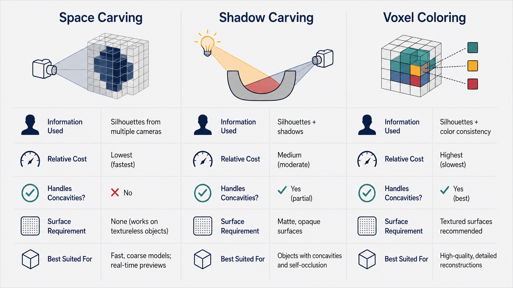
The three volumetric methods each occupy a distinct niche, defined by their assumptions, information source, and capabilities:
Space carving uses only silhouettes. It is the simplest and fastest of the three (per view), requires only the ability to segment the object from its background, and produces a conservative visual hull. It cannot recover concavities and degrades when silhouettes are imprecise. Best suited for convex or near-convex objects where silhouette segmentation is easy.
Shadow carving adds self-shadows to the silhouette consistency. It is more expensive (scales as $N+1$ times space carving with $N$ lights) but can recover some concave geometry that space carving misses. It requires a controlled lighting environment and fails for reflective or dark surfaces. Best suited for objects with complex concave geometry under controlled lab conditions.
Voxel coloring uses color consistency instead of silhouette geometry. It captures both shape and texture simultaneously, handles a wider variety of surface geometries than space carving (including concavities, provided they are photometrically distinct), and produces intrinsically textured reconstructions. It requires Lambertian surfaces and a specific camera ordering constraint. Best suited for objects with rich, matte surface texture.
All three are volumetric in the sense that they work within a bounded working volume, making them best suited for isolated object reconstruction rather than large-scale scene reconstruction. None of them replace structure from motion for recovering large environments.
Active Stereo vs. Volumetric Stereo: When to Use What
These two families of techniques address the correspondence problem in entirely different ways, and each excels in different scenarios.
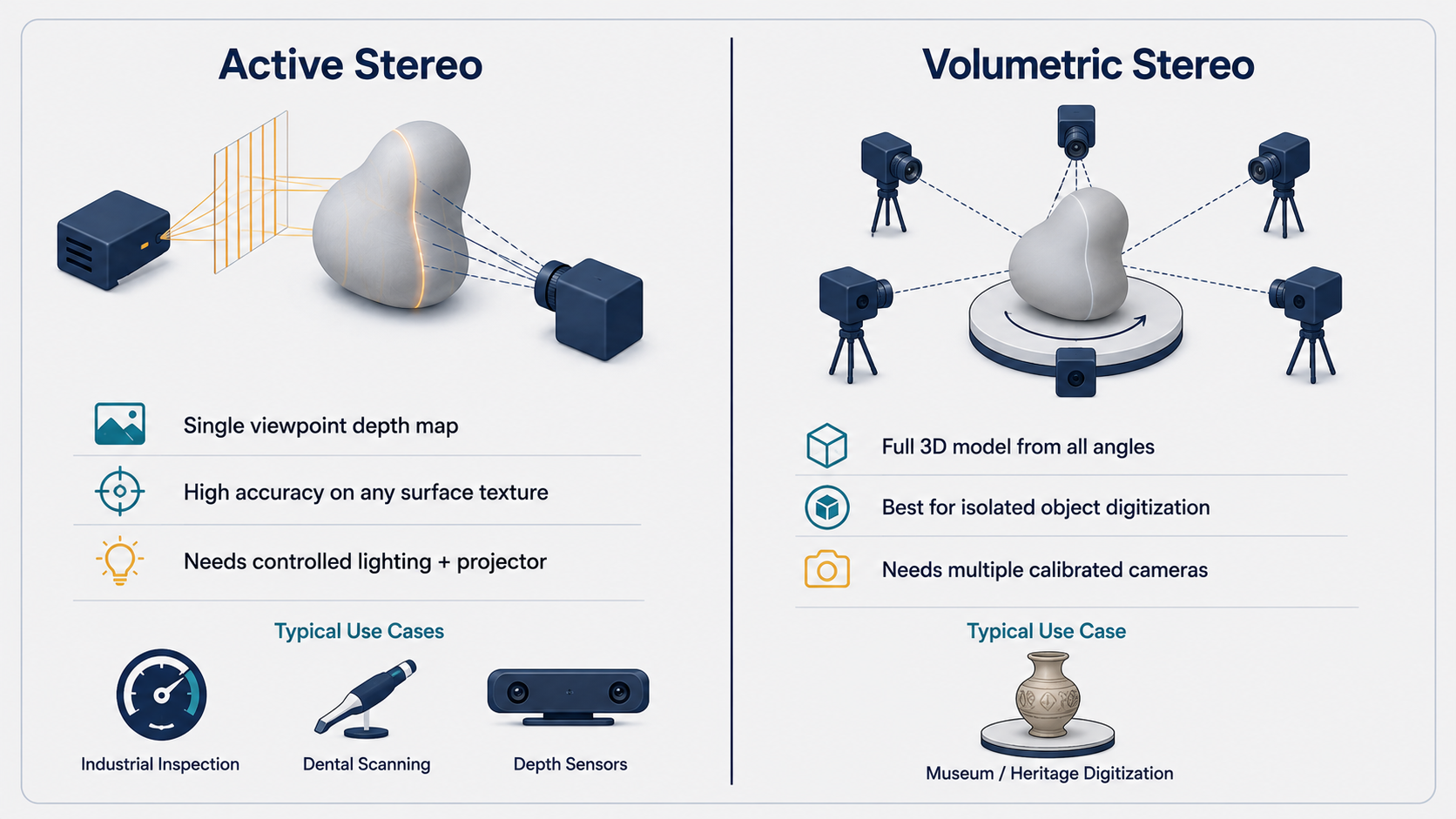
Active stereo — whether scanning stripe, structured light, or infrared dot patterns — is the right choice when you have control of the illumination and need high accuracy on arbitrary surfaces, including those with uniform texture or complex material properties. Industrial inspection systems, dental scanners, and consumer depth cameras (like the Kinect and its successors) all use active stereo precisely because it produces dense, accurate depth maps in challenging conditions. The trade-off is the need for a projector, controlled lighting, and the limitation that the projected pattern can interfere with simultaneously capturing natural-light photographs.
Volumetric stereo is the right choice when you can surround the object with multiple cameras and want a full 3D model rather than a depth map from a single viewpoint. It is particularly natural for object digitization — putting a sculpture or artifact on a turntable and photographing or filming it from all angles. The working volume assumption is naturally satisfied, and the resulting voxel representation can be directly converted to a mesh for rendering or analysis.
In the modern landscape, these approaches complement rather than replace each other. A sophisticated 3D scanning system might use structured light for high-accuracy depth from individual viewpoints, and then use volumetric or structure-from-motion methods to fuse multiple viewpoints into a coherent full-object model.
Conclusion: Rethinking the Problem to Solve It
What makes active and volumetric stereo conceptually satisfying is that they do not merely solve the correspondence problem — they reframe it.
Active stereo eliminates ambiguity by construction: projecting a known pattern ensures that the “which pixel matches which?” question has a trivially readable answer. You do not need to rely on the scene to be textured; you bring your own texture in the form of light. The practical consequences are enormous — from museum-quality digital archives of irreplaceable sculptures to depth-sensing capabilities in everyday consumer devices.
Volumetric stereo takes the inverse approach, questioning the very direction in which the problem is posed. Instead of working forward from image pixels to 3D points, it works backward from candidate 3D points to image consistency. The correspondence problem disappears because you are checking consistency directly in 3D, bypassing the 2D matching step entirely. The three variants — space carving, shadow carving, and voxel coloring — show how much mileage you can extract from different notions of consistency: geometric (silhouette), illumination-based (shadows), and photometric (color).
Taken together, these methods illustrate a broader lesson in computer vision: when a problem seems intractable, sometimes the right response is not a better algorithm for the original formulation, but a reframing of the problem itself. Projecting light to create correspondences, or checking candidate volumes rather than finding matches — both are examples of this creative reframing, and both have proven their worth in the lab and in the real world.
This article is based on CS231A Course Notes 5: Active and Volumetric Stereo, by Kenji Hata and Silvio Savarese, Stanford University.
Citation
If you found this useful, please cite this as:Patil, Aniket (May 2026). Active and Volumetric Stereo. https://AniketP04.github.io.
or as a BibTeX entry:
@article{patil2026active-and-volumetric-stereo,
  title   = {Active and Volumetric Stereo},
  author  = {Patil, Aniket},
  year    = {2026},
  month   = {May},
  url     = {https://AniketP04.github.io/blog/2026/Active_and_Volumetric_Stereo/}
}
Enjoy Reading This Article?
Here are some more articles you might like to read next: