How Machines Learn to See: A Deep Dive into Representations and Representation Learning

How Machines Learn to See: A Deep Dive into Representations and Representation Learning

From joint angles to latent vectors — why the way you describe the world determines everything a robot or AI system can do with it.

There is a question that sits quietly at the heart of all artificial intelligence: what is the right way to describe a situation? Before a robot can act, before a self-driving car can steer, before an image classifier can name what it sees — someone, or something, has to decide how to represent the information at hand. This choice, which sounds almost philosophical, turns out to have deeply practical consequences. A poor representation makes everything harder. A good one can make a seemingly intractable problem straightforward.

This essay is about representations — what they are, why they matter, how they were built by hand for decades, and how modern machine learning has learned to construct them automatically from raw data. Along the way, we will build intuition for the mathematical frameworks that underpin these ideas, including Markov chains, hidden Markov models, autoencoders, and the distinction between generative and discriminative models. These are not just abstract concepts — they are the conceptual infrastructure of modern robotics and computer vision.

Part 1: What Is a State, and How Do We Represent It?

The Concept of State

Imagine a walking robot — a two-legged machine striding across a flat surface. To reason about this robot, to predict where it will be a moment from now, or to decide what command to send its motors, you need some description of the robot’s current condition. This description is called the state of the system.

The state is not the physical robot itself. It is a compressed, symbolic summary of the aspects of the system that are relevant for the task at hand. For our walking robot, the state might include the angles of every joint, the angular velocity of each limb, the position and orientation of the robot’s torso in space, and its forward velocity. Fixed properties like limb lengths or joint friction are parameters, not state — they don’t change over time.

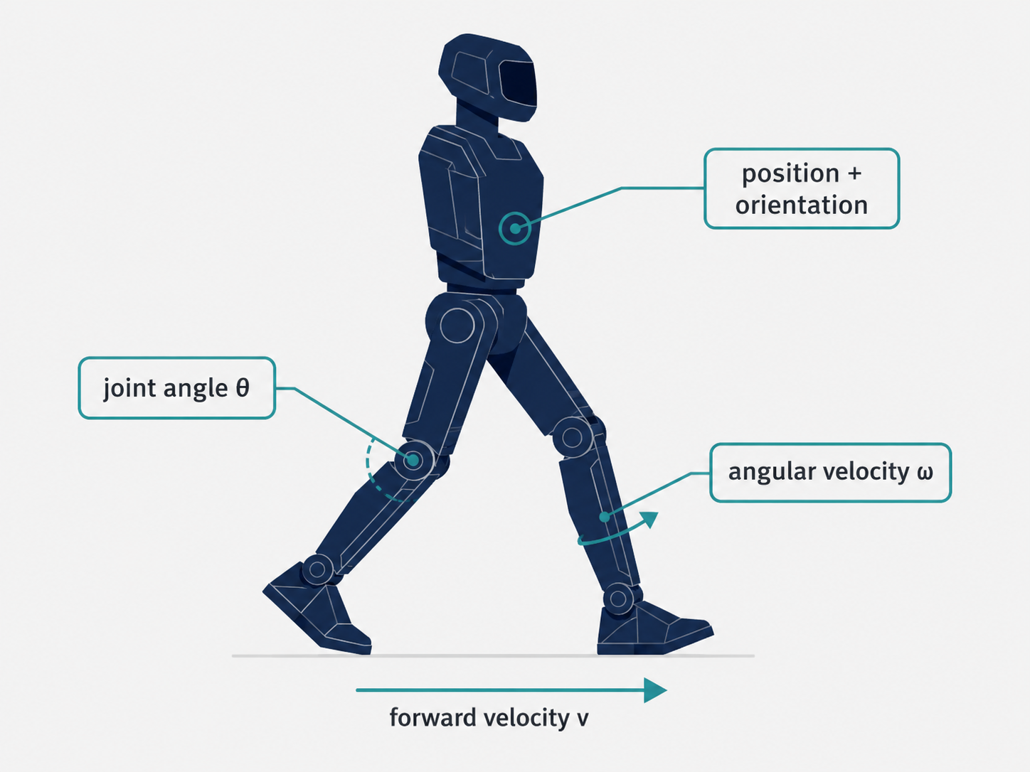
Here is the first key insight: the same physical system can be described by many different states, and the choice of which state to use is a design decision with real consequences. The orientation of the robot’s body, for instance, could be represented as Euler angles (three numbers describing rotations around three axes), as an axis-angle pair, or as a quaternion (a four-dimensional complex-number-like object that has nicer mathematical properties and avoids a phenomenon called gimbal lock). Each representation has different numerical properties, different computational costs, and different suitability for different downstream algorithms.

The same is true for positions (Cartesian versus polar coordinates), velocities, and almost any other physical quantity. Which representation is best depends on what you’re going to do with it.

Systems That Change Over Time

Real systems don’t sit still — they evolve. We denote the state at time $t$ as $x_t$. To predict the future, we need a model of how the state changes: a dynamics model $f$ such that $f(x_t) = x_{t+1}$.

For a robot joint, this might be quite concrete: if we know the current angular velocity, we can predict the joint angle at the next timestep. The dynamics function $f(\cdot)$ can be nonlinear and complex, but the structure is the same: the present state determines the next state.

The Markov Property — Why the Present Is Enough

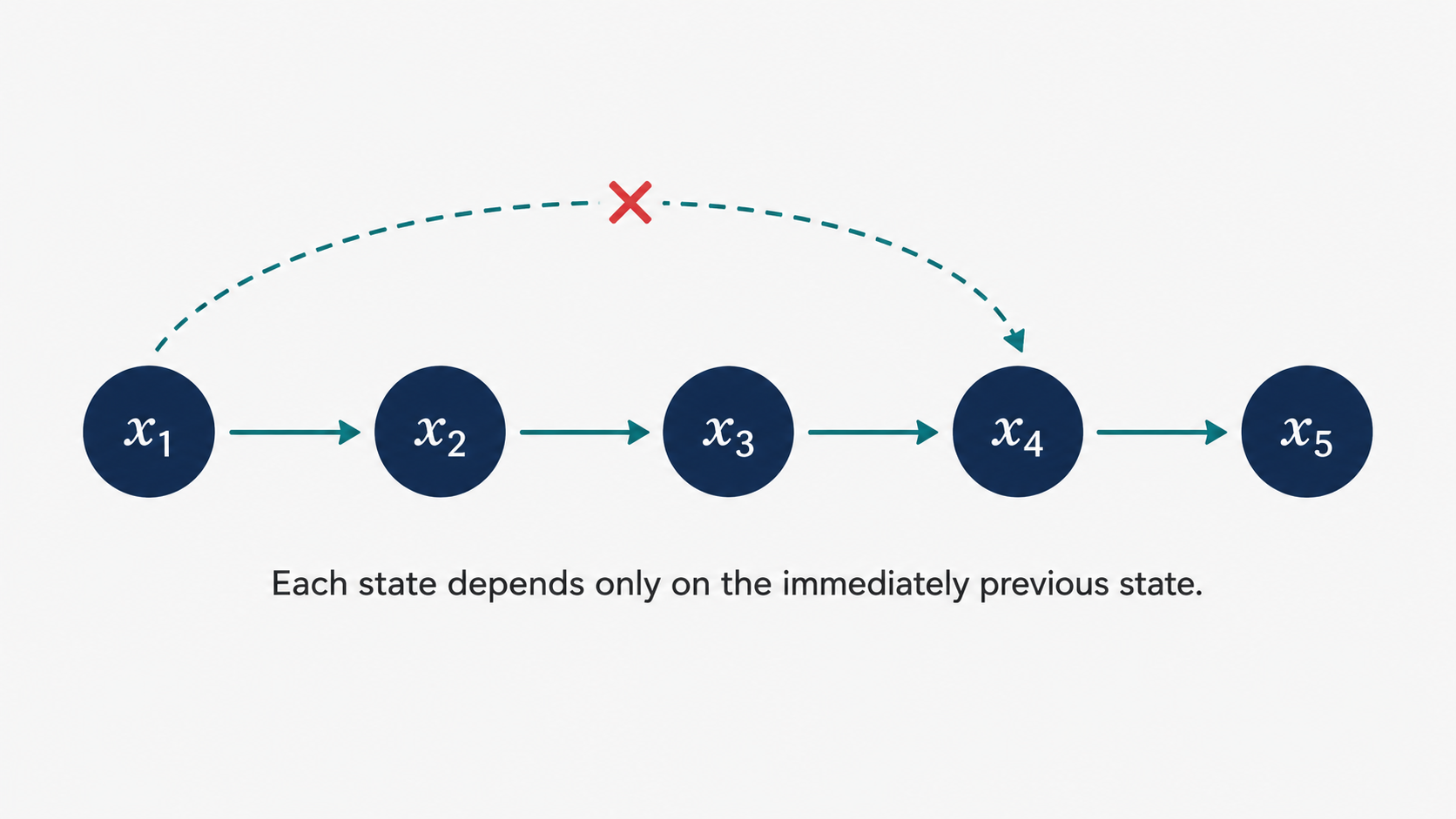
There is a crucial simplifying assumption that underlies most of the mathematical machinery in this space: the Markov property. It states that the future depends only on the present, not on how we got here. Formally:

\[P(x_{t+1} \mid x_t, x_{t-1}, \ldots, x_2, x_1) = P(x_{t+1} \mid x_t)\]

This is a profound claim. It says that once you know the current state $x_t$, the entire history $x_1, x_2, \ldots, x_{t-1}$ becomes irrelevant for predicting $x_{t+1}$. The state “summarizes” all the past information that matters for the future.

Is the Markov property always true in practice? Not necessarily — a robot’s current joint angle might not tell you everything about its trajectory if there’s unmodeled history (like accumulated fatigue or temperature effects). But it is a tremendously useful approximation, and choosing a state representation that makes the Markov property approximately true is itself part of good state design. A system that includes both position and velocity is more likely to be Markovian than one that tracks only position, since knowing “where I am and how fast I’m moving” is usually sufficient to predict “where I’ll be next.”

Systems that evolve with the Markov property are called Markov chains, and they are visualized as a sequence of state nodes where each node depends only on its immediate predecessor — a clean chain of causal influence through time.

When the State Is Hidden: Observations and Estimation

Markov chains assume we can directly observe the state $x_t$ at each timestep. But in practice, this is rarely true. A robot doesn’t “know” its joint angles — it reads them from noisy sensors. A self-driving car doesn’t directly perceive the 3D positions and velocities of surrounding vehicles — it receives raw camera frames and LiDAR point clouds and must infer those quantities.

This is the problem of state estimation: recovering the true (hidden) state from noisy, indirect observations. The appropriate model is the Hidden Markov Model (HMM), which adds an observation layer on top of the Markov chain. The states $x_t$ evolve as a Markov process, but we only see observations $z_t$ (sensor readings, images, etc.), where each observation depends only on the current state:

\[P(z_t \mid x_t, x_{t-1}, \ldots, x_1) = P(z_t \mid x_t)\]

The function $h(x_t) = z_t$ is called the observation model — it describes how the hidden state generates what we actually measure. For a camera on a self-driving car, $h$ is essentially the projection function mapping 3D world positions to 2D image pixels.

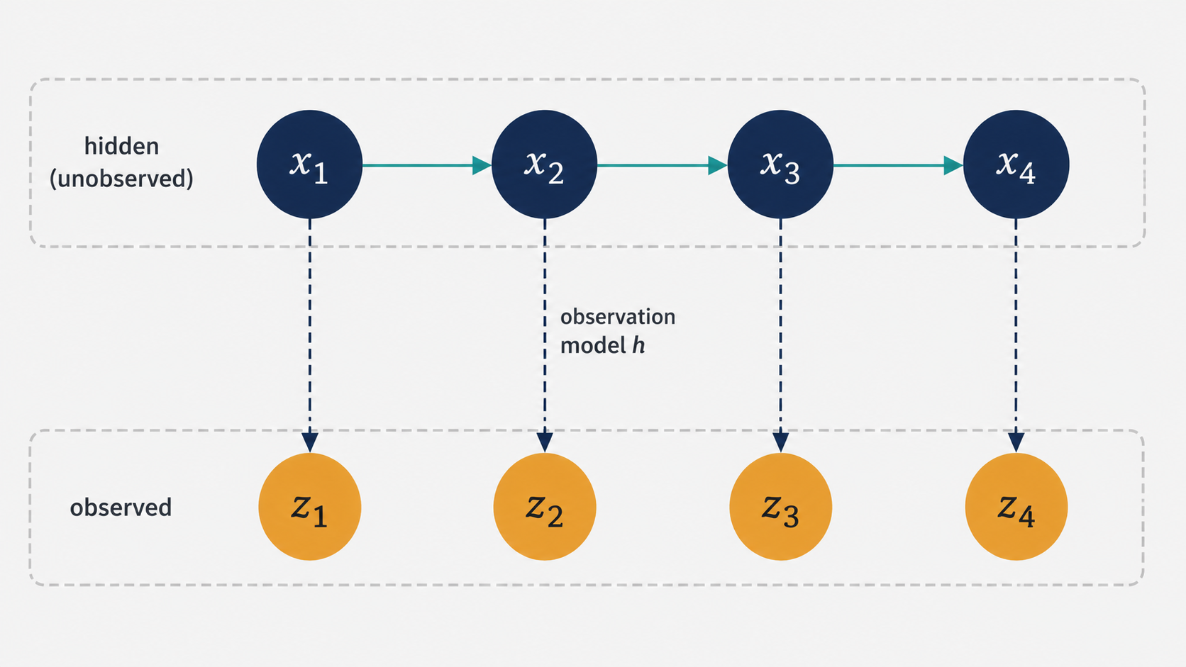
This two-layer structure — hidden states evolving according to dynamics, observed through a noisy sensor model — is one of the most widely applicable models in all of engineering. From GPS-aided navigation to speech recognition to visual tracking, HMMs and their extensions appear everywhere.

Adding Actions: The Full Decision-Making Picture

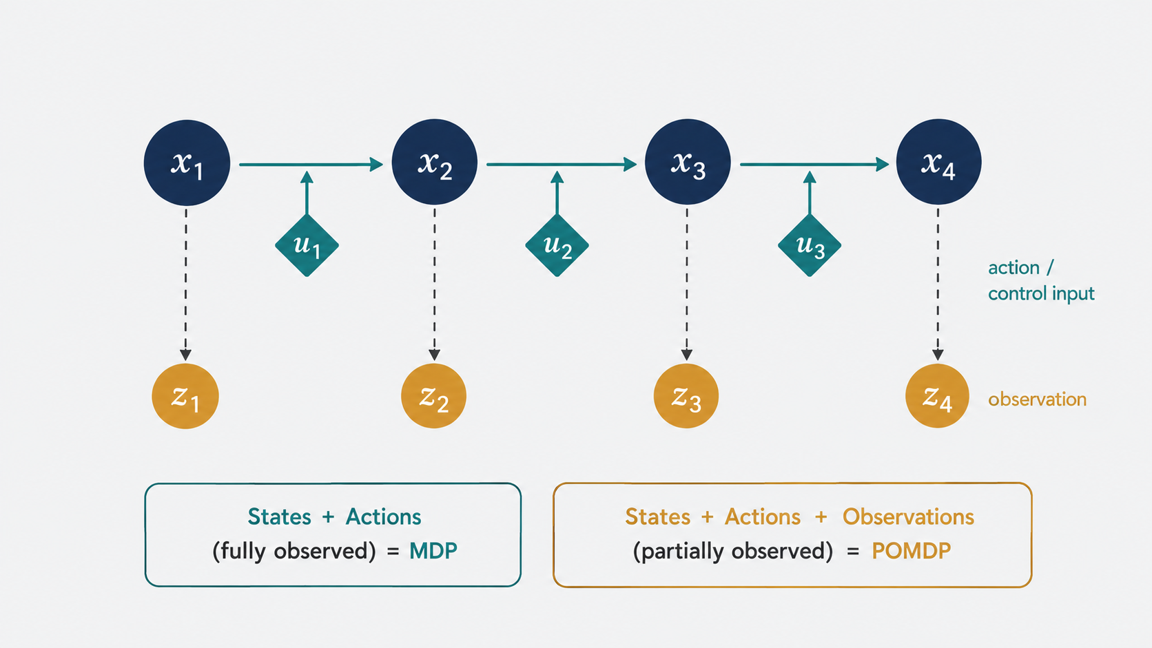
The HMM framework becomes even richer when we add a third element: control inputs. Instead of the dynamics being $f(x_t) = x_{t+1}$, we have $f(x_t, u_t) = x_{t+1}$, where $u_t$ is the action taken by the agent at time $t$. For the walking robot, $u_t$ might be the torque commands sent to each joint motor. For the self-driving car, it might be steering angle and throttle.

This extension transforms the Markov chain into a Markov Decision Process (MDP), and the HMM into a Partially Observable MDP (POMDP). The central question of these frameworks is no longer just “what is the current state?” but “what action should I take?” — the problem of decision-making under uncertainty. This is the foundation of reinforcement learning and optimal control, though exploring those areas fully is a separate journey.

Part 2: Generative vs. Discriminative Approaches to State Estimation

Two Fundamentally Different Philosophies

Once we have the HMM framework in hand — states, observations, dynamics, and observation models — the question becomes practical: given an observation $z$ (say, a camera image), how do we estimate the state $x$ (say, the 6D pose of an object in the scene)?

There are two philosophically distinct approaches, and understanding their difference is essential to understanding modern machine learning.

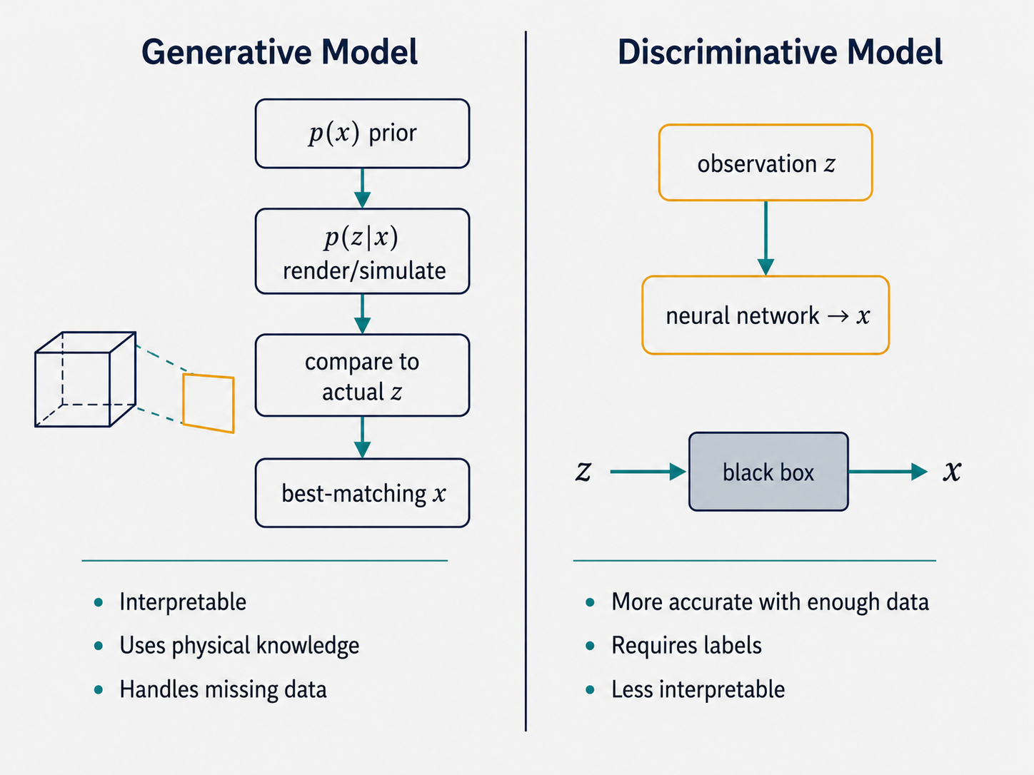
A generative model asks: what joint probability distribution $p(z, x)$ describes how observations and states co-occur? To use Bayes’ rule, this factors as $p(z, x) = p(z \mid x) \cdot p(x)$, where $p(z \mid x)$ is the observation likelihood (how likely is this image given this pose?) and $p(x)$ is a prior over states (how likely is this pose in the first place?). To estimate the pose from an image, you can sample candidate poses from the prior, use the observation model to “render” what the scene would look like in each pose, and find the candidate that best matches the actual image. The generative model is modeling the process by which observations are created.

A discriminative model takes a more direct approach. Instead of modeling how the world generates observations, it directly models the conditional probability $p(x \mid z)$ — given this observation, what is the state? You train a function (nowadays almost always a neural network) to map directly from input image to output pose. PoseCNN, for instance, takes an RGB image as input and outputs semantic labels, 3D translation estimates, and 3D rotation estimates simultaneously. The discriminative model doesn’t need to know how images are generated — it just needs to learn the mapping from image to answer.

The tradeoff is a classic one in machine learning. Generative models are more interpretable and can leverage physical knowledge (e.g., the laws of optics tell us how a 3D object projects onto a 2D image). They can also generate new data and handle missing information more gracefully. Discriminative models tend to be more accurate on their target task when trained on sufficient data, because they don’t waste capacity modeling aspects of the world irrelevant to the prediction — but they can be black boxes, and they typically require labeled data.

Part 3: What Is a Representation, Really?

The Three Layers of a Computer Vision Pipeline

Now we turn to a more specific and modern question: in the context of computer vision and machine learning, what exactly do we mean by a “representation,” and why does it matter so much?

Consider a complete vision pipeline. On one end, you have raw sensor data — a $1920 \times 1080$ RGB image, a depth map, a LiDAR point cloud. This is the input representation: the format in which raw perceptual data arrives. On the other end, you have whatever the system needs to produce — a class label (“fish”), a bounding box, a 6D pose, a segmentation mask. This is the output representation: a compact, task-specific summary of what matters for downstream decision-making.

In between these two ends sits the most interesting layer: the intermediate representation. This is a compressed, low-dimensional encoding of the high-dimensional input that captures the information necessary to derive the output. In a deep neural network, the intermediate representation is the activation vector at some internal layer — a dense numerical vector, perhaps of dimension 512 or 2048, that summarizes the content of the input image in a form the output layer can use.

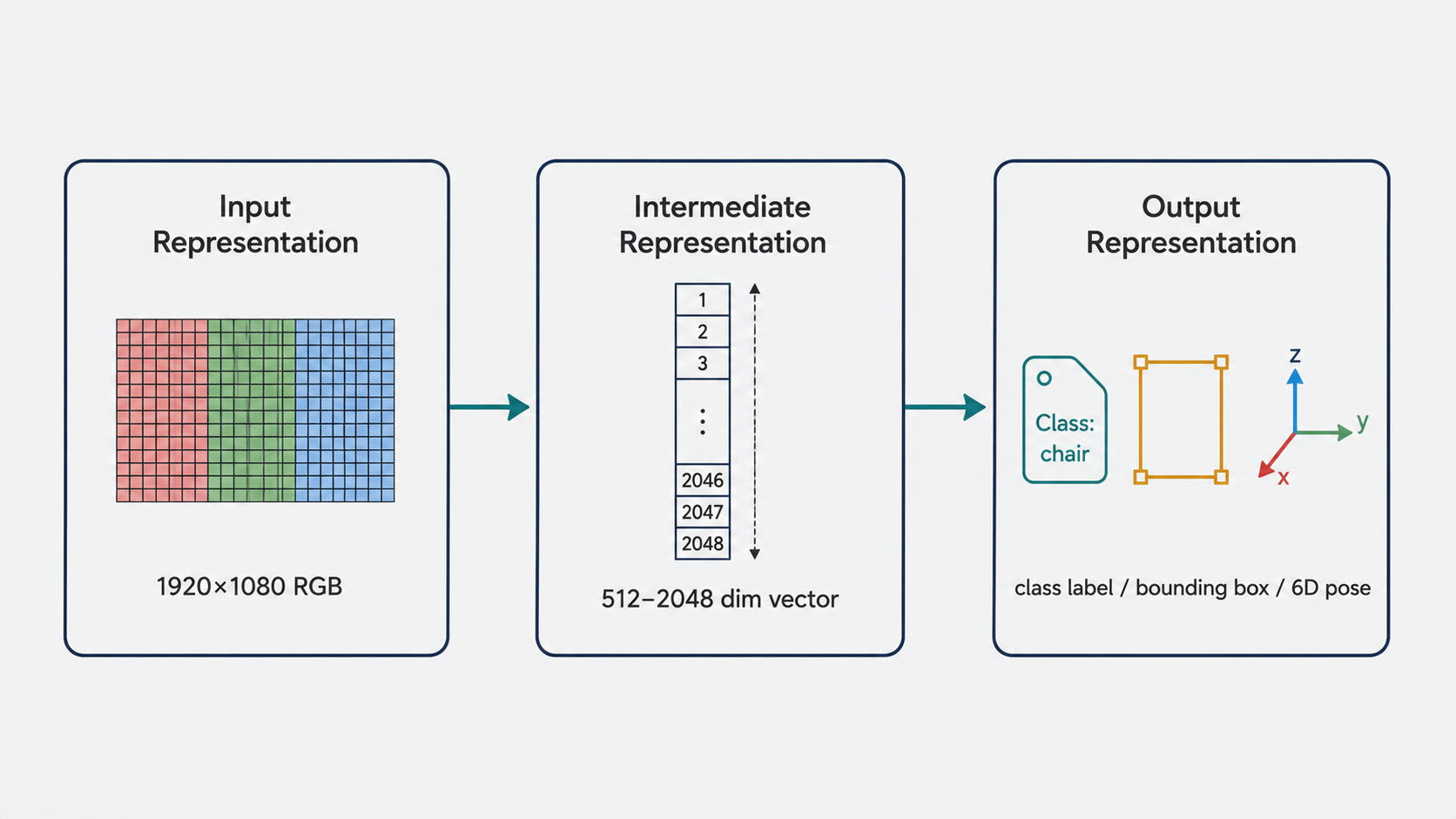
The intermediate representation is where most of the intellectual action happens in modern computer vision, because it is here that raw pixels are transformed into something semantically meaningful. How this transformation happens — whether by hand or by learning — is the central story of the last decade of computer vision research.

What Makes a Good Representation?

This is not just a practical question but a theoretical one, and Yoshua Bengio and colleagues have articulated a set of properties that a good representation should ideally satisfy.

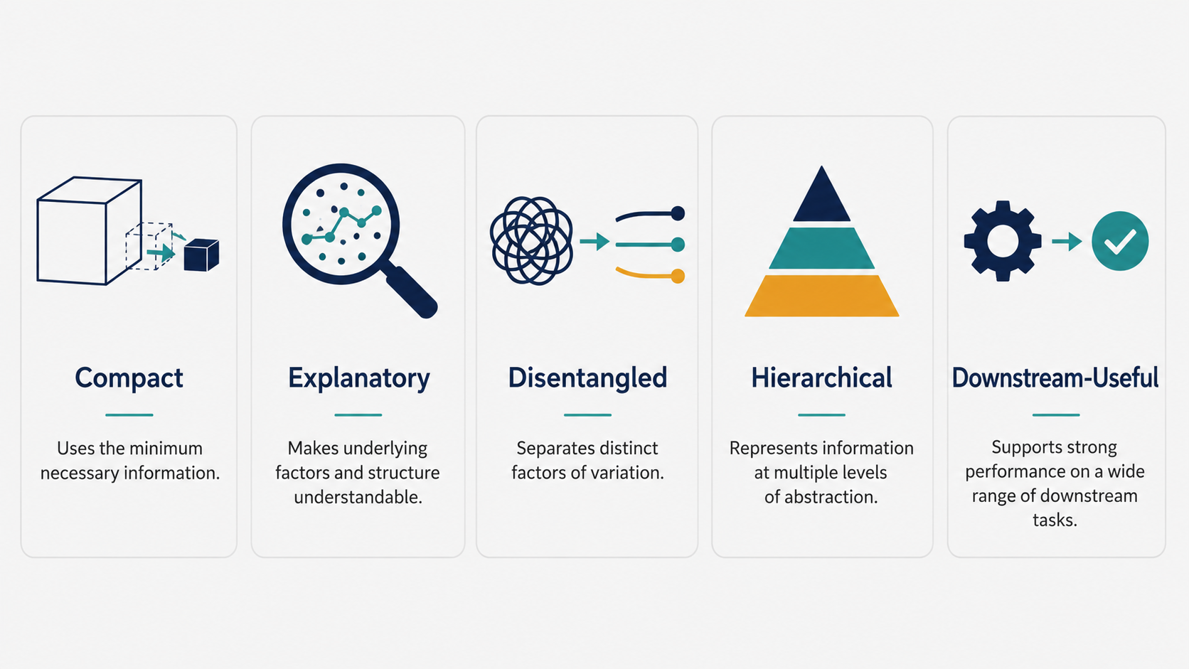
A good representation should be compact: it should use as few dimensions as possible. A $1920 \times 1080$ RGB image contains roughly 6 million numbers. Most of those numbers are redundant — neighboring pixels are correlated, the background is uninformative, the color distribution is constrained. A compact representation discards this redundancy and retains only what matters.

At the same time, it must be explanatory — expressive enough to capture the full range of relevant variation in the input. A representation that collapses all images to a single number is perfectly compact but useless. The tension between compactness and expressiveness is the fundamental challenge of representation design.

A good representation should also be disentangled. This means that different factors of variation in the world — an object’s shape, its color, its position, the lighting — should be encoded in different, independent parts of the representation. If you change the lighting in a scene, a disentangled representation should change only in the “lighting” dimensions, leaving the “object identity” dimensions unchanged. Disentanglement makes representations more generalizable, more interpretable, and more useful for downstream tasks that may care about only some factors.

The property of being hierarchical reflects the observation that the world has structure at multiple scales. Edges compose into textures, textures into parts, parts into objects, objects into scenes. A good representation captures this hierarchy, allowing low-level features to be reused in the construction of high-level concepts — much as the same edge detector is useful for recognizing both dogs and cars, even though those are very different categories.

Finally, and most pragmatically, a good representation should make downstream tasks easier. This is ultimately the ground truth criterion: does using this representation improve the accuracy, efficiency, or robustness of the classification, detection, or control system that consumes it? The quality of a representation can always be measured, at least indirectly, by the downstream performance it enables.

Part 4: Hand-Crafted Representations — The Classical Era

The Philosophy of Feature Engineering

For most of the history of computer vision (roughly up to 2012), intermediate representations were designed by humans. The process was called feature engineering or feature extraction, and it occupied a large fraction of the field’s intellectual energy.

The philosophy was intuitive: if you want to recognize a clownfish, you reason about what makes a clownfish visually distinctive — its orange and white stripes, its particular body shape, its characteristic fin structure. You then design mathematical operations on the image that detect these properties: edge detectors to find stripe boundaries, color histograms to capture the orange-white distribution, texture descriptors to characterize surface patterns. The result is a vector of numbers — a feature descriptor — that encodes these human-defined properties.

This hand-crafted intermediate representation is then fed into a classifier (a support vector machine, a decision tree, or a simple neural network) that learns to map from the feature vector to a class label. The two stages — feature extraction and classification — were largely separate.

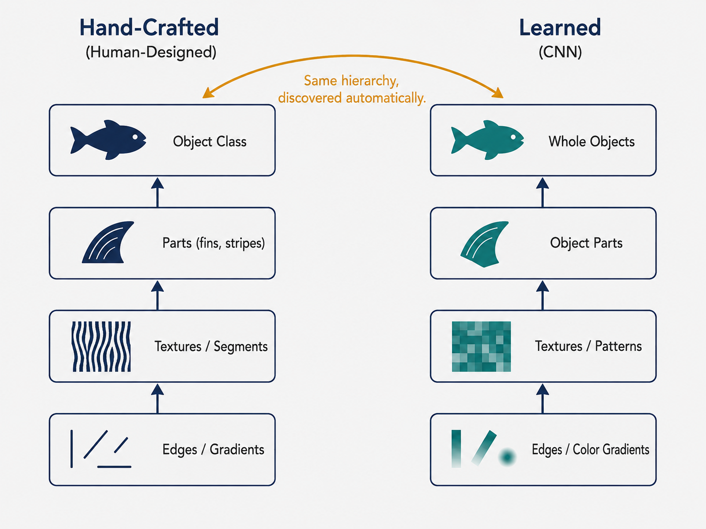
The pipeline had a natural hierarchical structure. Low-level features (raw edges, color gradients) were combined into mid-level features (segments, textures), which were combined into high-level features (parts, body plan), which were used to make the final prediction. This mirrors the way humans describe visual objects: a clownfish has fins (part), which have stripes (texture), which have sharp color boundaries (edges).

The Strengths and Limits of Hand-Crafted Features

The primary virtue of hand-crafted representations is interpretability. Because a human designed every feature, a human can explain why it matters. If a classifier rejects an image as “not a clownfish,” you can trace back through the features and understand what was missing — perhaps the color histogram didn’t have enough orange, or the edge detector didn’t find the expected stripe pattern. In high-stakes domains — medical imaging, legal evidence analysis, safety-critical robotics — this transparency can be essential.

The limitations, however, are severe. Designing good features requires deep domain expertise. It is slow, laborious, and often produces features that are brittle: they work well in the conditions for which they were designed but fail when the lighting changes, the viewing angle shifts, or the object is partially occluded. And crucially, the features are designed to capture what humans think is relevant, which may not align with what is actually most predictive.

For tasks where human intuition is a good guide, hand-crafted features work surprisingly well. For tasks where the relevant patterns are subtle, high-dimensional, or not easily articulable in human terms — like distinguishing malignant from benign tissue in a histology slide, or estimating the emotional state of a pedestrian from their gait — hand-crafted features simply can’t compete.

Part 5: Learned Representations — The Modern Era

The Neural Network Revolution

Around 2012, a shift occurred that is now widely recognized as one of the most dramatic transitions in the history of machine learning. Driven by the combination of large labeled datasets (like ImageNet, with over a million labeled images), cheap parallel computation (GPUs), and algorithmic improvements to deep neural networks — most importantly, the systematic training of deep convolutional architectures — learned representations displaced hand-crafted ones as the dominant paradigm in computer vision.

The key idea is simple to state but profound in its implications: instead of designing the intermediate representation by hand, you train a neural network end-to-end, and let the learning process discover the representation automatically. The convolutional layers of the network learn to act as feature extractors — but the features they learn are optimized for the task at hand, not for what a human engineer thought was important.

The result, empirically, was a dramatic improvement in accuracy across nearly every vision benchmark. Networks trained on ImageNet achieved error rates that human-engineered systems could not approach.

What Do Neural Networks Actually Learn?

This success raises an immediate question: what, exactly, are the learned features? They are not designed to be interpretable, and the activations of internal layers are just large vectors of numbers. Can we understand them?

Zeiler and Fergus, in a landmark 2014 paper, visualized the learned representations of a deep CNN trained on ImageNet by finding the input image patches that maximally activated each filter at each layer. Their discovery was striking and somewhat surprising: the learned representations were hierarchical in the same way as the hand-crafted ones. Early layers in the network responded to simple edges and color gradients. Middle layers responded to textures and patterns. Deeper layers responded to object parts — eyes, wheels, faces — and the deepest layers responded to entire objects.

This convergence suggests that the hierarchical structure of good representations is not just a human design preference — it is, in some sense, the correct structure for visual understanding, one that learning discovers on its own when given enough data and capacity. The hand-crafted pipelines were approximating the right answer; the learned ones found it more precisely.

Visualizing the Learned Space with t-SNE

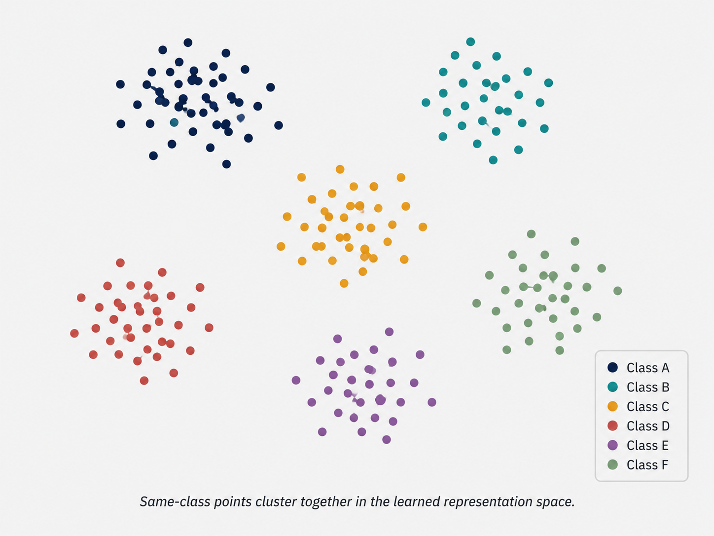
Another window into learned representations is dimensionality reduction. The intermediate representation of a trained neural network is a high-dimensional vector (perhaps 2048 dimensions for a modern ResNet). We can’t directly visualize 2048 dimensions, but we can project them down to 2D for inspection using t-SNE (t-distributed Stochastic Neighbor Embeddings).

t-SNE works by minimizing the KL divergence between a probability distribution over pairs of points in high-dimensional space (where “probability” reflects similarity — nearby points have high probability) and the corresponding distribution in 2D space. The result is a 2D map where nearby points in the original high-dimensional representation end up nearby in the 2D visualization.

When applied to the intermediate representations of a well-trained CNN, the t-SNE plot reveals that images of the same class cluster together, even across considerable visual variation. Images of the digit “3” from MNIST, written in many different handwriting styles, all land in the same region of the 2D map. This is powerful evidence that the learned representation has captured something genuinely semantic — “three-ness” — rather than superficial pixel statistics. The representation has disentangled the identity of the digit from the style of its rendering.

Part 6: Learning Without Labels — Autoencoders and Self-Supervised Learning

The Label Bottleneck

Supervised learning requires labeled data. For image classification, every training image needs a class label. For pose estimation, every training image needs a 6D pose annotation. For object detection, every image needs bounding boxes. Acquiring these labels is expensive: it requires human annotators, domain expertise, and time. A medical dataset might require a specialist to label each image; a robotics dataset might require expensive motion-capture equipment.

Meanwhile, unlabeled data is essentially free. Every camera ever deployed generates a continuous stream of images. Every robot generates a continuous stream of sensor readings. The question becomes: can we learn meaningful representations from this ocean of unlabeled data?

The answer, developed over the past decade and now central to modern AI, is yes.

The Autoencoder: Learning by Compression

The autoencoder is the foundational idea for unsupervised representation learning. Its architecture is symmetric: an encoder network compresses the input $\mathbf{X}$ (say, an image) into a low-dimensional intermediate representation $\mathbf{z}$, and a decoder network attempts to reconstruct the original input from $\mathbf{z}$, producing $\hat{\mathbf{X}} = \mathcal{F}(\mathbf{X})$.

The training objective is simply to minimize the reconstruction loss — the difference between the input and its reconstruction:

\[\arg\min_{\mathcal{F}} \mathbb{E}_{\mathbf{X}} \left[ \| \mathcal{F}(\mathbf{X}) - \mathbf{X} \| \right]\]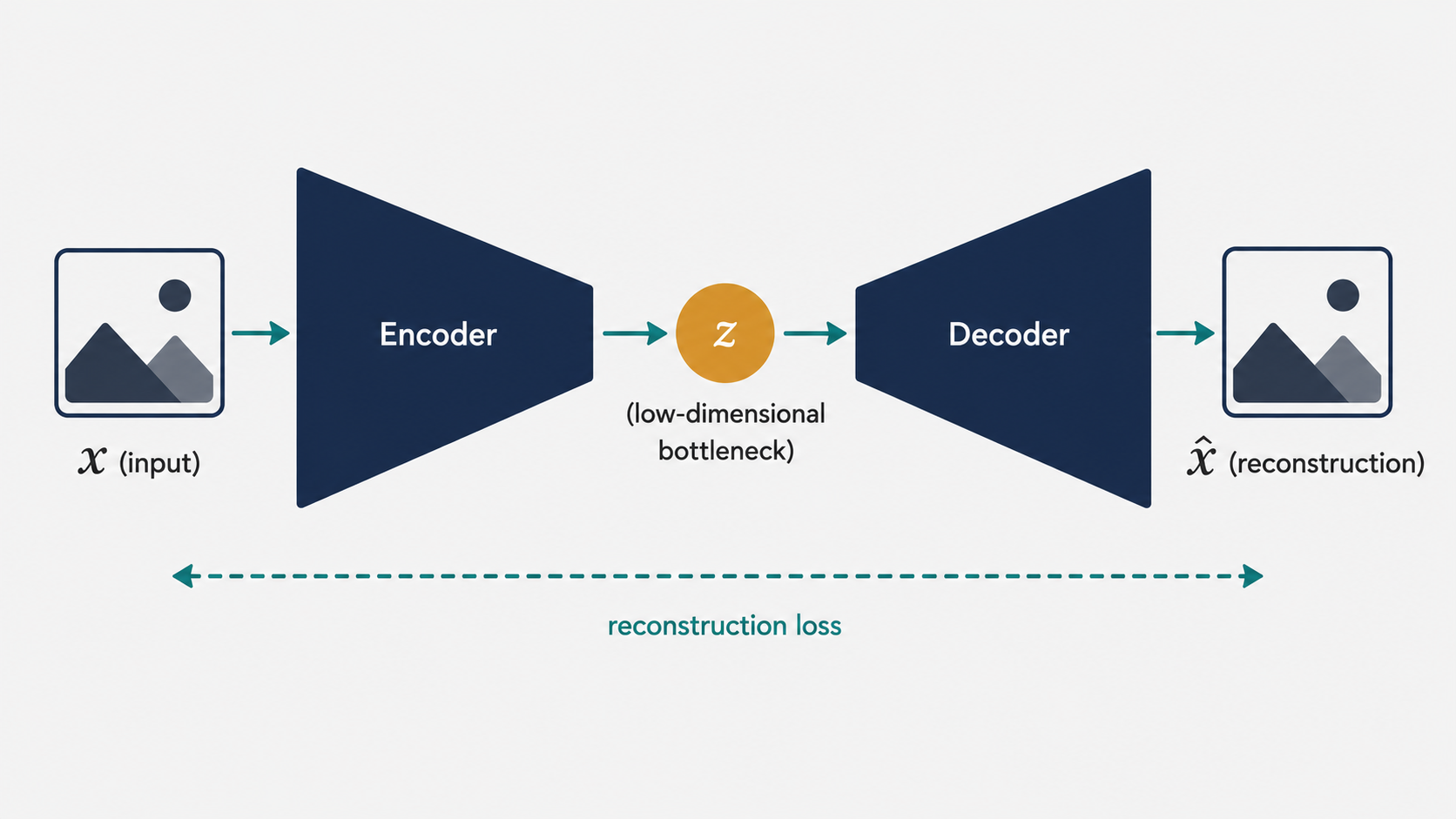

No external labels are needed. The input image itself serves as the training target.

The magic lies in the bottleneck. The intermediate representation $\mathbf{z}$ has far fewer dimensions than the input $\mathbf{X}$. To successfully reconstruct $\mathbf{X}$ from $\mathbf{z}$, the encoder must learn to compress the most important information about $\mathbf{X}$ into those few dimensions. Redundant information (background noise, uninformative correlations) gets discarded; the information that distinguishes one input from another must be preserved. This is exactly the kind of compact, explanatory representation we want.

Concretely: if you train an autoencoder on a dataset of face images, the bottleneck representation $\mathbf{z}$ will likely encode attributes like identity, expression, pose, and lighting — because these are the factors that vary across faces and that the decoder needs in order to reconstruct the image. Factors that are constant across all images (like “has two eyes and a nose”) don’t need to be in $\mathbf{z}$ because the decoder can learn them as default assumptions.

The encoder half of a trained autoencoder is a powerful, general-purpose feature extractor. It can be applied to new images to produce compact representations, which can then be used as inputs to downstream classifiers or other models. And it was trained entirely without labels.

Self-Supervised Learning: Creating Your Own Labels

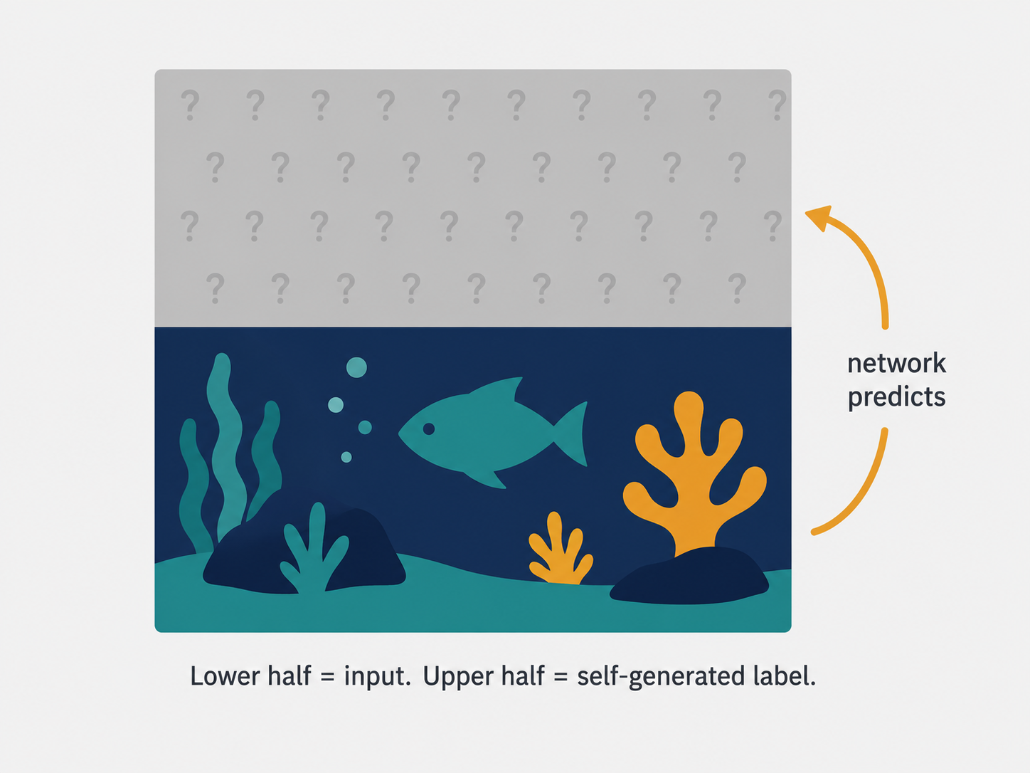
Self-supervised learning extends this idea further by creating synthetic training targets from the data itself, without any human annotation. The key move is to deliberately withhold part of the input and ask the model to predict the missing part.

In one simple example, take an image, hide the upper half, and ask the network to reconstruct the upper half given the lower half. The lower triangle of pixels is the input; the upper triangle is the label — generated automatically from the same image. No human annotation required.

The intuition is that to successfully predict the missing region, the network must understand the semantic content of the image at some level. A model that has truly understood “this is a fish swimming near coral” can make a reasonable prediction about what the top of the image looks like, even though it hasn’t seen it. A model that has memorized pixel statistics without understanding content cannot.

This idea, seemingly simple, has produced some of the most powerful models in modern AI. The BERT family of language models is trained by masking random words and predicting them from context. The MAE (Masked Autoencoder) for images masks large random patches of an image and trains the model to reconstruct them. These self-supervised objectives, applied at scale, produce representations that transfer remarkably well to downstream tasks — often matching or exceeding the performance of supervised methods trained on large labeled datasets.

The Transfer Learning Payoff

What makes unsupervised and self-supervised pre-training so valuable in practice is the concept of transfer learning. The workflow proceeds in two stages:

First, train the encoder (or the full self-supervised model) on a large unlabeled dataset. This pre-training phase is computationally expensive but can be done once and the result shared broadly. The model learns a rich, general-purpose intermediate representation.

Second, for a specific downstream task (say, medical image classification), collect a small labeled dataset — perhaps a few thousand examples, which is far cheaper to annotate than millions. Train a lightweight classifier on top of the frozen (or lightly fine-tuned) encoder. Because the encoder has already learned to produce meaningful, compact representations, the classifier needs very little data to achieve high accuracy.

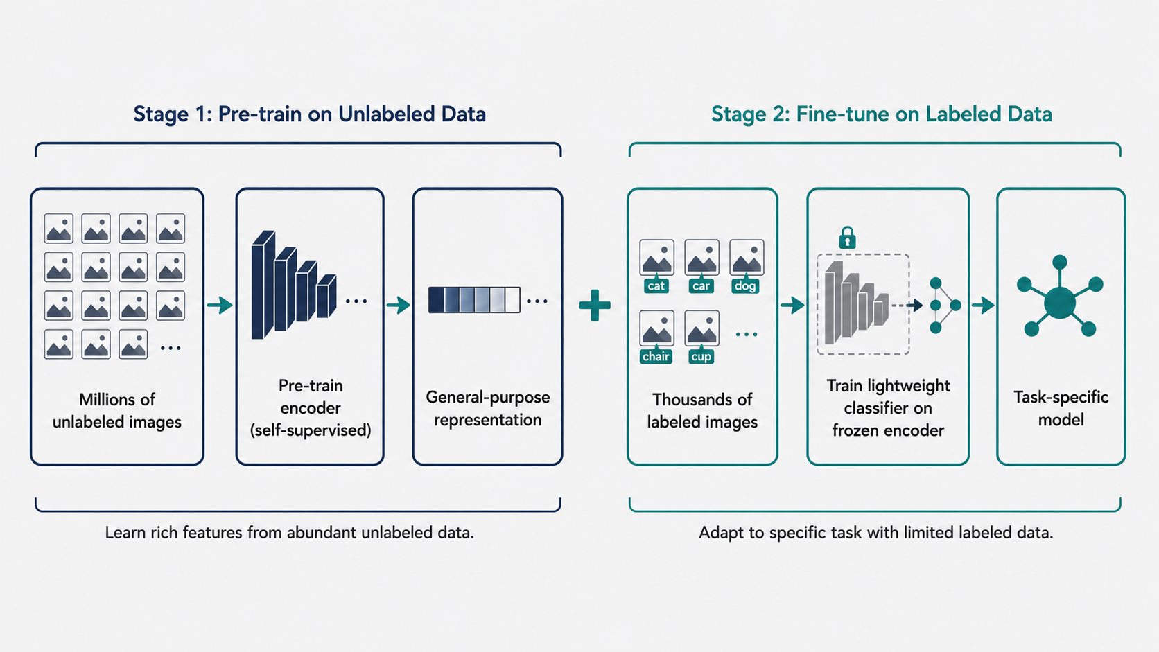
This two-stage approach has become the dominant paradigm in modern AI. The large-scale pre-training provides the “representational foundation,” and the small labeled dataset provides the task-specific “finishing touches.” It is representation learning in its most practically powerful form.

Conclusion: The Representation Is the Intelligence

Looking across the full arc of this essay — from walking robots and Markov chains, through the hand-crafted features of classical computer vision, to learned representations and self-supervised autoencoders — a unifying theme emerges. The way you represent information is not a minor implementation detail. It is, in a deep sense, the intelligence itself.

A perfect state representation that satisfies the Markov property allows simple dynamics models to make accurate predictions. A compact, disentangled intermediate representation allows a simple classifier to generalize robustly. A rich, hierarchical learned representation allows a model trained on one task to transfer to another with minimal additional data. In each case, the quality of the representation determines the ceiling on what the downstream system can achieve.

The evolution from hand-crafted to learned representations is not the story of humans becoming unnecessary — it is the story of human insight being applied at a higher level of abstraction. Rather than designing features, we now design learning objectives (reconstruction loss, mask prediction, contrastive similarity), architectures (convolutional networks, transformers), and training regimes. The features emerge automatically, and they turn out to be better than what we could have designed by hand — because the data contains patterns that our intuitions don’t anticipate.

The question “what is the right representation?” remains as central and difficult as ever. But we now have powerful tools for answering it empirically — by training, evaluating, visualizing, and iterating. Understanding these tools, and the conceptual framework that connects states, observations, generative models, and learned features, is the foundation for everything that follows in modern robotics and computer vision.

This article is based on CS231A Course Notes 7: Representations and Representation Learning, by Kenji Hata and Silvio Savarese, Stanford University.

Representations and Representation Learning