What a Single Photograph Knows About the World: A Deep Dive into Single View Metrology

What a Single Photograph Knows About the World: A Deep Dive into Single View Metrology

How vanishing points, lines at infinity, and projective geometry allow us to reconstruct 3D structure — and even calibrate a camera — from a single image.

There is something quietly remarkable about the photograph you took of a city street last summer. The buildings recede into the distance, the parallel lanes of the road appear to converge at a point on the horizon, and without thinking about it, your brain instantly interprets the entire scene as three-dimensional. You know the buildings are rectangular, the road lanes are parallel, and the architecture is roughly perpendicular. But how does your brain do this from a flat, two-dimensional image? And more importantly — can a computer do the same thing, with mathematical rigor?

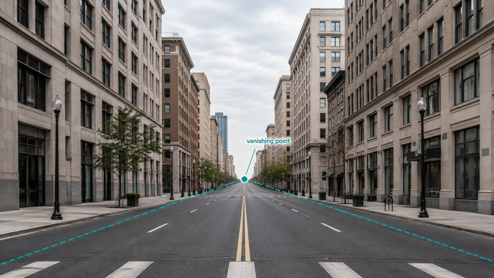
This is the central question of single view metrology: given only one photograph and (ideally) some knowledge of the camera that took it, how much geometric information about the 3D world can we recover? The answer, it turns out, is a surprising amount. We can deduce the orientations of planes, the directions of lines, the angles between surfaces, and even calibrate the camera itself — all without ever pointing a ruler at the real world.

To understand how this works, we need to build up a vocabulary of ideas, starting from the mathematics of transformations in 2D, moving through the elegant concept of “points at infinity,” and culminating in the powerful machinery of vanishing points and horizon lines that let us reason about 3D geometry from flat pictures.

Part 1: A Hierarchy of Transformations — What Gets Preserved and What Doesn’t

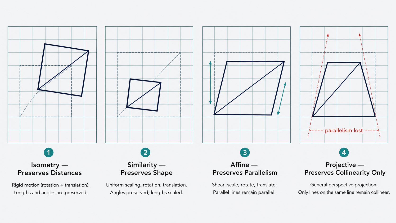
Before asking what a camera destroys when it projects the 3D world onto a 2D image, it helps to have a precise vocabulary for the kinds of transformations that exist and what each one preserves. Think of this as a ladder of increasingly permissive transformations, each rung sacrificing some geometric property in exchange for more flexibility.

Isometries: The Rigid Body

An isometric transformation is the most restrictive kind — it preserves distances. If you pick up a rigid object and move it around without bending or stretching it, you’ve performed an isometry. The object can rotate and translate, but nothing else. Mathematically, using homogeneous coordinates (where a 2D point $(x, y)$ is represented as the triple $(x, y, 1)^T$ for reasons we’ll appreciate shortly), an isometry looks like:

\[\begin{pmatrix} x' \\ y' \\ 1 \end{pmatrix} = \begin{pmatrix} R & t \\ 0 & 1 \end{pmatrix} \begin{pmatrix} x \\ y \\ 1 \end{pmatrix}\]

Here, $R$ is a $2 \times 2$ rotation matrix and $t$ is a $2 \times 1$ translation vector. Because distances are preserved, so are angles, areas, and shapes — everything you’d expect from a rigid transformation.

Similarities: Adding Scale

A similarity transformation relaxes isometries by allowing uniform scaling. A photocopy machine that enlarges or shrinks an image while keeping its shape intact is a physical analogy. The formula adds a scalar $s$ multiplied against the rotation:

\[\begin{pmatrix} x' \\ y' \\ 1 \end{pmatrix} = \begin{pmatrix} sR & t \\ 0 & 1 \end{pmatrix} \begin{pmatrix} x \\ y \\ 1 \end{pmatrix}, \quad S = \begin{pmatrix} s & 0 \\ 0 & s \end{pmatrix}\]

Similarity transformations preserve shape, which means they preserve angles and ratios of lengths, even if they don’t preserve lengths themselves. Every isometry is a special similarity where $s = 1$, but not every similarity is an isometry.

Affine Transformations: Stretching and Shearing

Affine transformations are more general still. They are defined as:

\[T(\mathbf{v}) = A\mathbf{v} + \mathbf{t}\]

where $A$ is any invertible linear transformation. In homogeneous coordinates:

\[\begin{pmatrix} x' \\ y' \\ 1 \end{pmatrix} = \begin{pmatrix} A & t \\ 0 & 1 \end{pmatrix} \begin{pmatrix} x \\ y \\ 1 \end{pmatrix}\]

Affine transformations can scale non-uniformly, shear, and stretch — think of what happens when you view a circle painted on the ground from an oblique angle: it becomes an ellipse. Yet affine transformations still preserve a key structural property: parallelism. If two lines were parallel before the transformation, they remain parallel after it. They also preserve straight lines and ratios of distances along a line.

Projective Transformations (Homographies): The Most General Case

The final and most general transformation is the projective transformation, also called a homography. In homogeneous coordinates:

\[\begin{pmatrix} x' \\ y' \\ w' \end{pmatrix} = \begin{pmatrix} A & t \\ v^T & b \end{pmatrix} \begin{pmatrix} x \\ y \\ 1 \end{pmatrix}\]

The key difference from the affine case is the extra row $\begin{pmatrix} v^T & b \end{pmatrix}$ at the bottom. This seemingly small addition has a dramatic effect: projective transformations do not preserve parallelism. This is precisely what makes them the right model for what a camera does. When you photograph a tiled floor, the parallel grout lines appear to converge toward a point in the image — a projective transformation has been applied.

What does a projective transformation preserve? Two things: collinearity (points on a line remain on a line — lines map to lines) and the cross-ratio of four collinear points, defined as:

\[\text{cross ratio} = \frac{\|P_3 - P_1\| \cdot \|P_4 - P_2\|}{\|P_3 - P_2\| \cdot \|P_4 - P_1\|}\]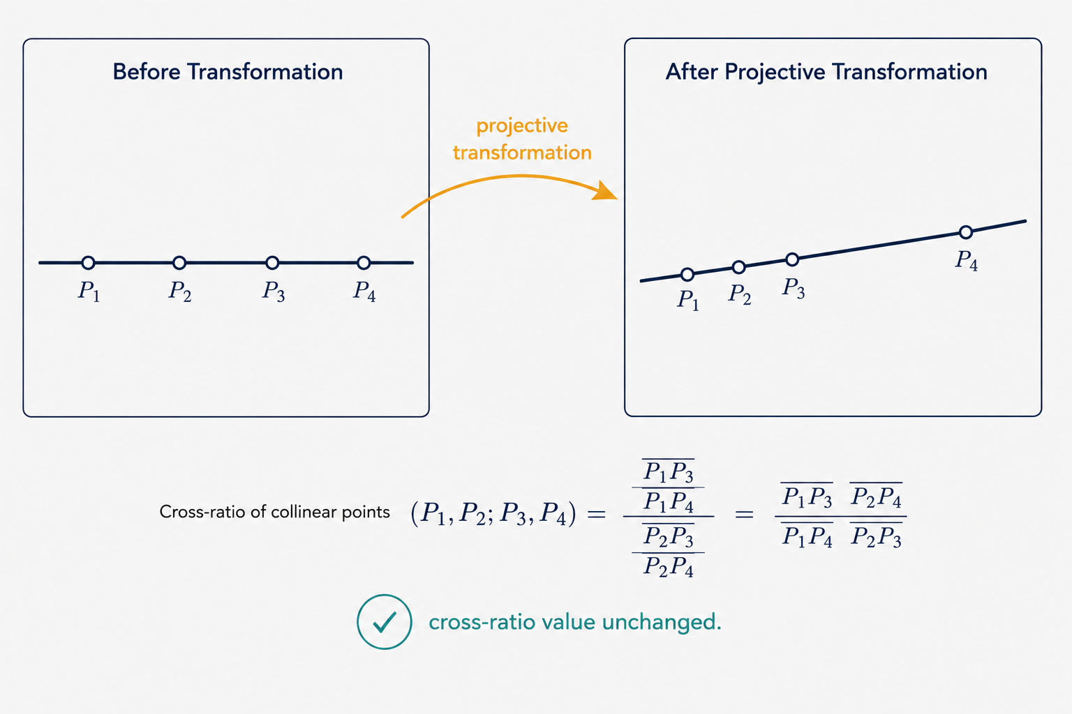

This cross-ratio is the deepest invariant of projective geometry — a number that doesn’t change no matter how you project or transform the four points, as long as their collinearity is maintained. It is the fingerprint that a projective transformation cannot alter.

—

Part 2: Points and Lines at Infinity — Where Parallel Lines “Meet”

Here’s a philosophical puzzle that has a beautiful mathematical resolution. Every student learns that parallel lines never intersect. And yet, when you stand on a long straight road and look toward the horizon, the road’s edges appear to converge to a single point. Which is it — do they meet or not?

The answer lies in the genius of homogeneous coordinates, which give us a unified framework to talk about both ordinary intersections and intersections “at infinity.”

Representing Lines in 2D

A line in 2D can be written as $ax + by + c = 0$, and in homogeneous form, it is represented by the vector $\ell = \begin{pmatrix} a & b & c \end{pmatrix}^T$. A point $\mathbf{p} = \begin{pmatrix} x & y & 1 \end{pmatrix}^T$ lies on the line if and only if $\ell^T \mathbf{p} = 0$. The ratio $-a/b$ captures the slope and $-c/b$ captures the y-intercept.

The intersection of two lines $\ell$ and $\ell’$ is elegantly given by their cross product: $\mathbf{x} = \ell \times \ell’$. You can verify this directly: by the definition of the cross product, $\mathbf{x}$ is orthogonal to both $\ell$ and $\ell’$, which in our notation means $\mathbf{x}^T \ell = 0$ and $\mathbf{x}^T \ell’ = 0$ — exactly the condition for $\mathbf{x}$ to lie on both lines.

The Beautiful Resolution: Ideal Points

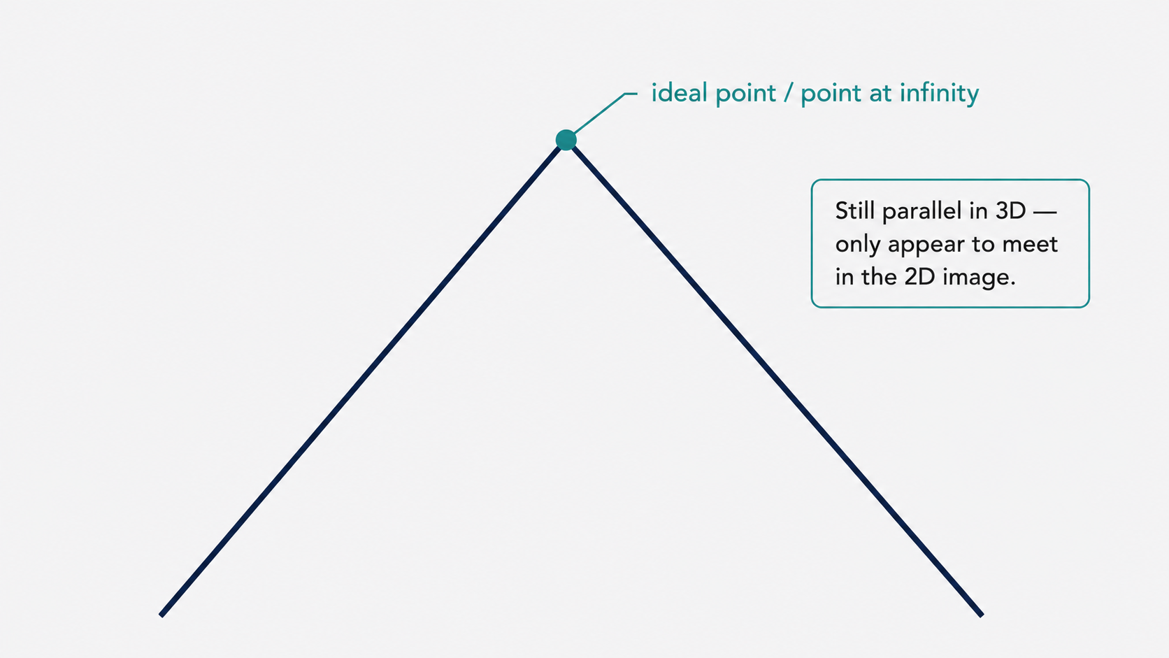
Now, what happens when two lines are parallel? Their slopes are equal, meaning $a/b = a’/b’$. Computing the cross product gives:

\[\ell \times \ell' \propto \begin{pmatrix} b \\ -a \\ 0 \end{pmatrix} = \mathbf{x}_\infty\]

Notice the last coordinate: it’s zero. In homogeneous coordinates, converting back to Euclidean coordinates requires dividing by the last coordinate. A zero last coordinate means the point is at infinity — formally, we’d be dividing by zero, which sends the point infinitely far away. This is called an ideal point or a point at infinity.

What makes this elegant is the consistency: every point of the form $(x, y, 0)^T$ in homogeneous coordinates represents a direction — a point infinitely far in that direction. And all parallel lines with slope $-a/b$ share the same ideal point $(b, -a, 0)^T$. You can verify: $\ell^T \mathbf{x}_\infty = a \cdot b + b \cdot (-a) + c \cdot 0 = 0$, so every parallel line in the family passes through that ideal point. This is the mathematical formalization of the intuition that parallel lines “meet at the horizon.”

The Line at Infinity

If we gather all the ideal points together — from every possible family of parallel lines — they all share a remarkable property: they lie on a single line at infinity, denoted $\ell_\infty$. We can define it as:

\[\ell_\infty = \begin{pmatrix} 0 & 0 & 1 \end{pmatrix}^T\]

You can verify: for any ideal point $(x, y, 0)^T$, we have $\ell_\infty^T \mathbf{x}_\infty = 0 \cdot x + 0 \cdot y + 1 \cdot 0 = 0$, so every ideal point lies on this line. The line at infinity is the mathematical home of all directions.

What Transformations Do to Points at Infinity

This is where the distinction between affine and projective transformations becomes crucially important.

Under a projective transformation $H$, a point at infinity $\mathbf{p}_\infty = (x, y, 0)^T$ gets mapped to:

\[\mathbf{p}' = H\mathbf{p}_\infty = \begin{pmatrix} A & t \\ v^T & b \end{pmatrix} \begin{pmatrix} x \\ y \\ 0 \end{pmatrix} = \begin{pmatrix} p'_x \\ p'_y \\ p'_z \end{pmatrix}\]

The last coordinate $p’_z = v^T (x, y)^T$ is generally nonzero, meaning the point at infinity has been mapped to an ordinary finite point. This is exactly what a camera does: it takes a direction (a point at infinity in the 3D world) and maps it to a specific pixel in the image. Parallel lines in 3D, sharing an ideal point, get mapped to lines in the image that converge at a real, observable pixel location.

Under an affine transformation, however, the bottom row is $(0, 0, 1)$, so the last coordinate of the transformed point is always $0 \cdot x + 0 \cdot y + 1 \cdot 0 = 0$. Affine transformations preserve the line at infinity: ideal points stay ideal, and parallelism is maintained.

Similarly, lines transform under projective transformations via $\ell’ = H^{-T} \ell$, and the line at infinity is not generally preserved by projective transformations (it gets mapped to some finite line in the image), but affine transformations do preserve it.

Part 3: Vanishing Points and Horizon Lines — The Window into 3D

We are now ready to make the leap from abstract 2D geometry into the 3D world and its relationship to images. This is where the theory becomes practically powerful.

Vanishing Points: Where the World’s Infinity Lands in Your Image

Imagine a long straight road stretching away from you. The road’s edges are parallel lines in 3D. Their ideal point — the point at infinity in the direction of the road — gets projected by the camera onto a real pixel in the image. That pixel is the vanishing point.

More precisely, suppose a family of parallel lines in 3D all run in direction $\mathbf{d} = (a, b, c)^T$ (in the camera’s coordinate frame). Their point at infinity in 3D is $(a, b, c, 0)^T$ in homogeneous 3D coordinates. The camera matrix $K$ (the intrinsic calibration matrix encoding focal length, principal point, etc.) projects this to an image point. The resulting vanishing point $\mathbf{v}$ in the image satisfies:

\[\mathbf{v} = K\mathbf{d}\]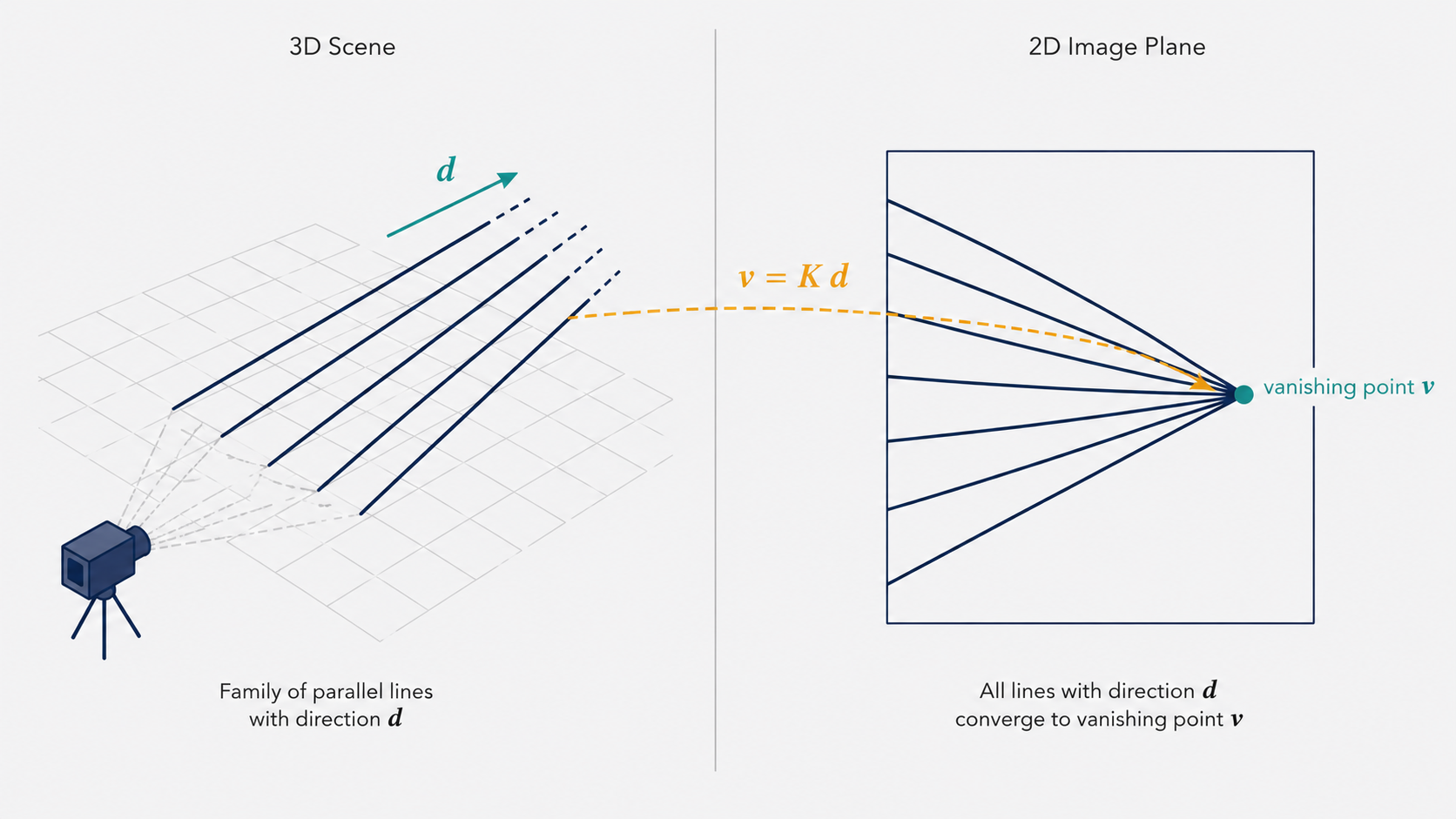

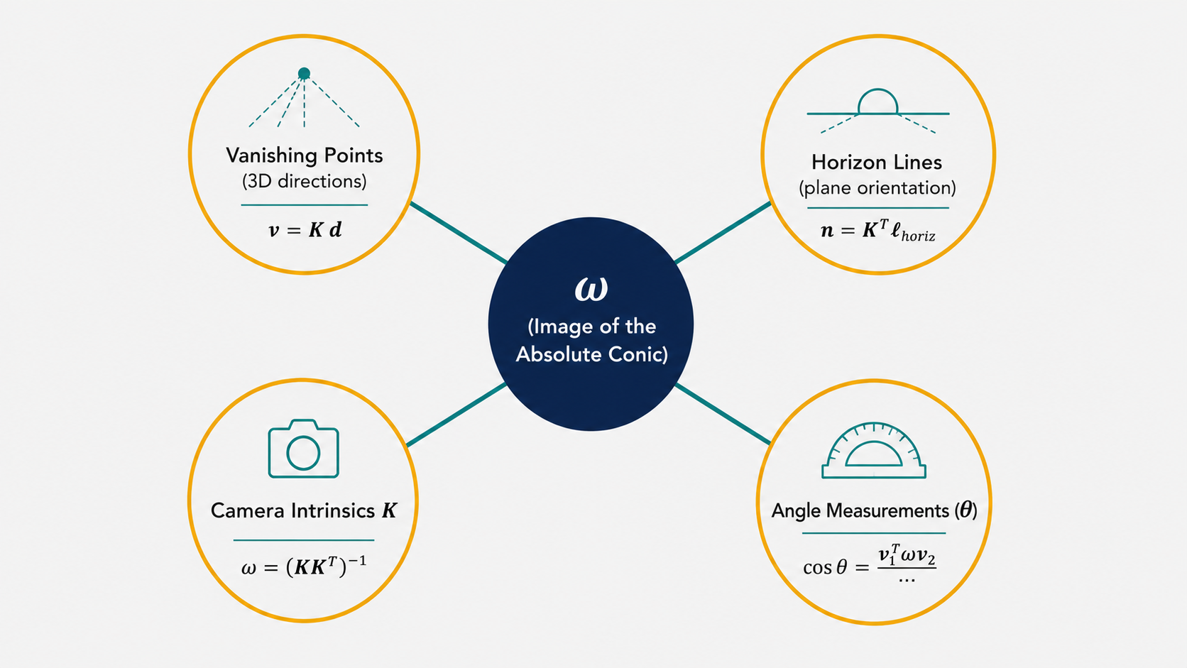
This is a strikingly simple equation. It says that the vanishing point of a family of parallel lines is completely determined by the direction of those lines and the camera’s intrinsic parameters. Conversely, if we observe a vanishing point $\mathbf{v}$ in the image and know $K$, we can recover the 3D direction:

\[\mathbf{d} = \frac{K^{-1}\mathbf{v}}{\|K^{-1}\mathbf{v}\|}\]

The normalization ensures $\mathbf{d}$ is a unit vector representing a pure direction in 3D space. This is a powerful inverse operation: by looking at where lines converge in a photograph, we can recover the actual orientation of those lines in the real world.

The Horizon Line: A Plane’s Signature in the Image

A single plane in 3D (think of a tiled floor, the face of a building, or the surface of a table) contains many families of parallel lines. Each family has its own vanishing point. The horizon line (or vanishing line) of the plane is the image-line that passes through all these vanishing points.

Here’s the intuition: all families of parallel lines within a plane share the same “line at infinity” in 3D (since they all lie in the plane). When the camera projects the scene, this line at infinity in the plane maps to a specific line in the image — the horizon line. Mathematically:

\[\ell_{\text{horiz}} = H_P^{-T} \ell_\infty\]

where $H_P$ is the projective transformation induced by the camera’s projection of that particular plane.

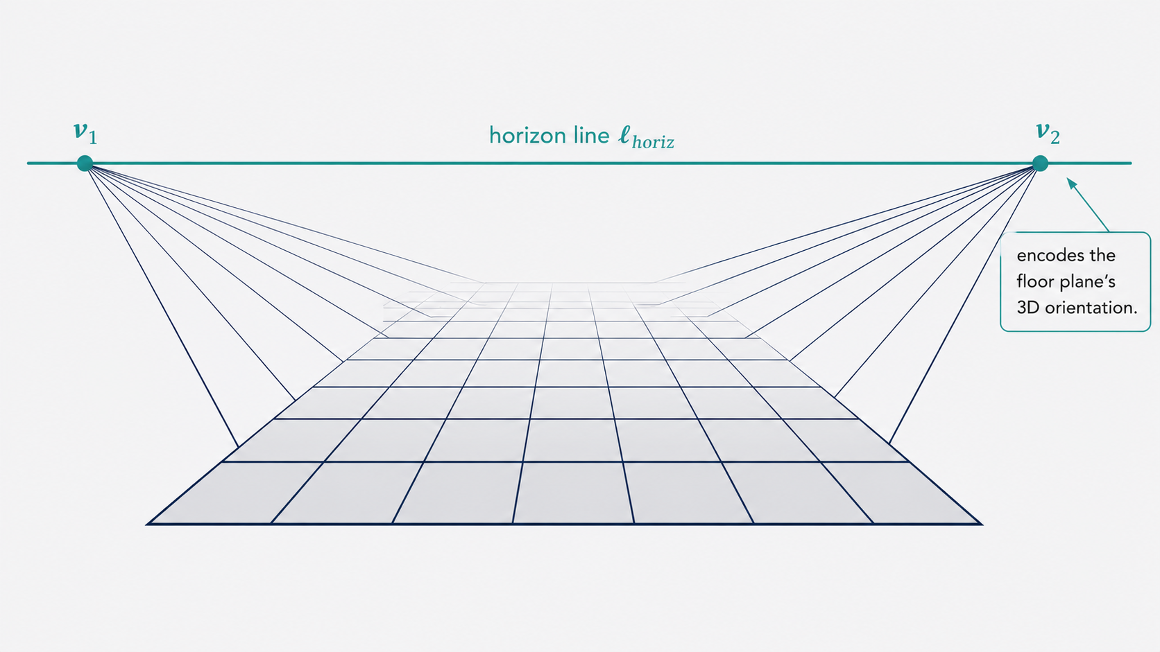
The practical power of the horizon line is remarkable. Think about looking at a photograph of a road: even though the lane markings clearly converge in the image, you know they are parallel in the real world. The horizon line is the mathematical tool that encodes this knowledge — it tells you which line in the image corresponds to “the direction of infinity” for all lines on that road surface.

Furthermore, the horizon line encodes the orientation of the plane in 3D. If the camera is calibrated (i.e., $K$ is known), then the normal vector $\mathbf{n}$ to the plane can be extracted directly from the horizon line:

\[\mathbf{n} = K^T \ell_{\text{horiz}}\]

This is a beautiful result. The horizon line in the image — a line you can literally see and identify — encodes the perpendicular direction to the plane in 3D space. If you can find the horizon line of the floor in a photograph, you immediately know which direction is “up” relative to that floor’s surface.

Measuring Angles Between Directions and Planes

The machinery we’ve built so far allows us to do something that might seem impossible at first: measure angles between lines and planes in 3D, using only their image projections.

Suppose two families of parallel lines in 3D have directions $\mathbf{d}_1$ and $\mathbf{d}_2$, corresponding to vanishing points $\mathbf{v}_1$ and $\mathbf{v}_2$ in the image. The angle $\theta$ between the directions is the angle whose cosine is $\mathbf{d}_1 \cdot \mathbf{d}_2 / (|\mathbf{d}_1| |\mathbf{d}_2|)$.

Substituting $\mathbf{d}_i = K^{-1}\mathbf{v}_i / |K^{-1}\mathbf{v}_i|$ and doing some algebra, this becomes:

\[\cos\theta = \frac{\mathbf{v}_1^T \omega \mathbf{v}_2}{\sqrt{\mathbf{v}_1^T \omega \mathbf{v}_1} \cdot \sqrt{\mathbf{v}_2^T \omega \mathbf{v}_2}}\]

where $\omega = (KK^T)^{-1}$. The matrix $\omega$ is called the image of the absolute conic (IAC) — it is a symmetric $3 \times 3$ matrix that encodes all of the camera’s intrinsic parameters in a form that is directly useful for computing angles.

Think of $\omega$ as a kind of “metric ruler” for the image plane. Ordinarily, angles in the image don’t correspond to angles in the 3D world (the camera distorts them). But $\omega$ provides the correction factor that translates image measurements back into real-world angular measurements.

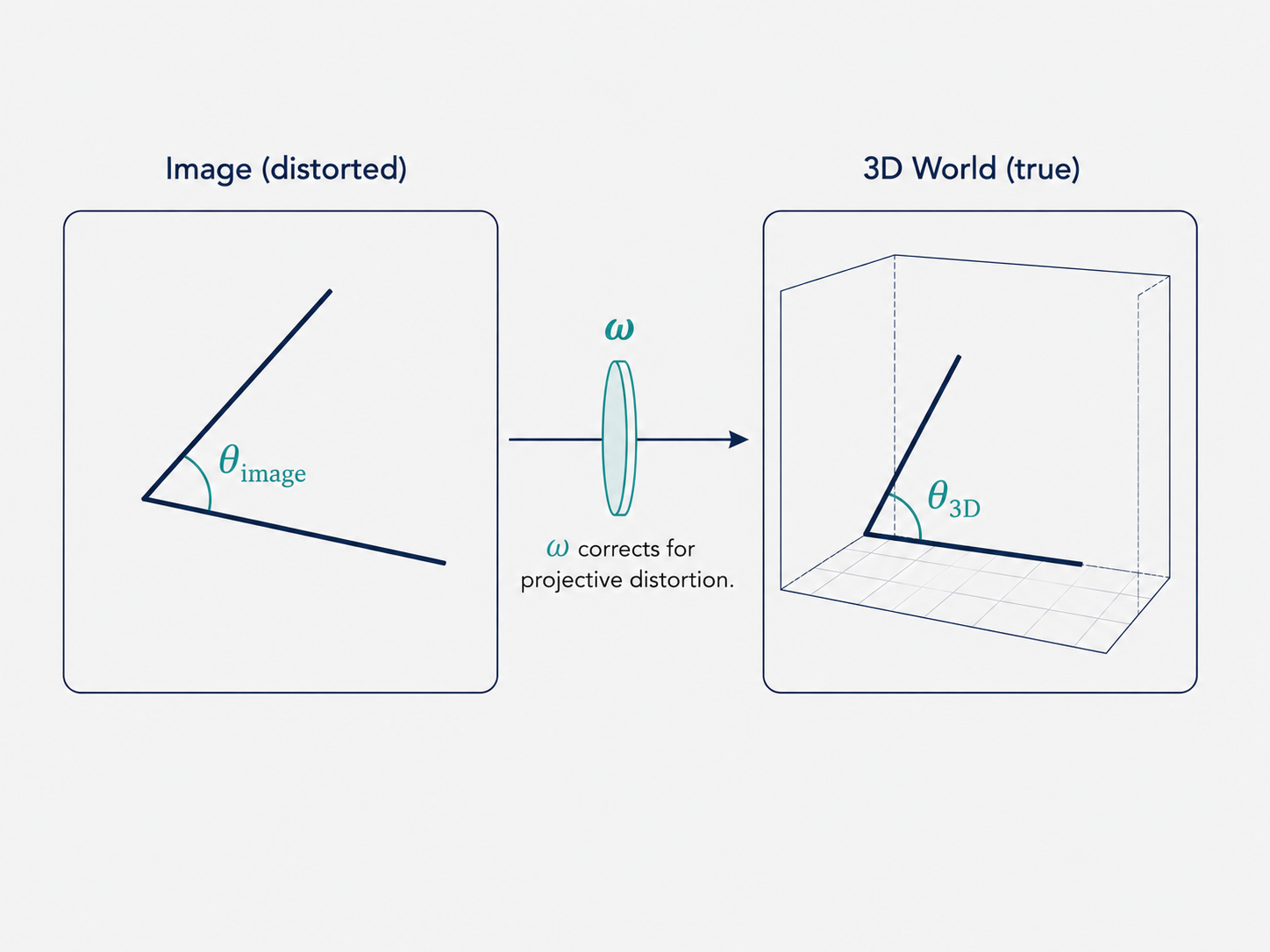
Analogously, the angle between two planes in 3D can be derived from their horizon lines $\ell_1$ and $\ell_2$:

\[\cos\theta = \frac{\ell_1^T \omega^{-1} \ell_2}{\sqrt{\ell_1^T \omega^{-1} \ell_1} \cdot \sqrt{\ell_2^T \omega^{-1} \ell_2}}\]

Both equations share the same fundamental structure: the matrix $\omega$ (or its inverse) acts as the metric that transforms the projective image coordinates into an inner product that reflects the true 3D geometry.

Part 4: Calibrating a Camera from a Single Image

Now we arrive at arguably the most remarkable application of everything we’ve developed. Normally, camera calibration requires a physical calibration target — a checkerboard pattern photographed from many angles, for instance. But what if we already have a single photograph of a structured scene, with no calibration target in sight? Can we recover the camera’s intrinsic parameters $K$ from the photograph alone?

The answer is yes, under certain conditions.

The Setup: Orthogonal Planes in the Scene

The key observation is that the constraint “$\cos\theta = 0$” (i.e., two lines or planes are perpendicular) is one of the most common geometric constraints we encounter in man-made environments. Buildings have walls that meet at right angles, rooms have floors and ceilings that are perpendicular to walls, and corridors contain edges that are mutually orthogonal. We can exploit this structure.

Suppose we identify two families of parallel lines in the image — one for each of two planes that we know (from context) are perpendicular in 3D. We extract the two vanishing points $\mathbf{v}_1$ and $\mathbf{v}_2$. Since the corresponding directions are perpendicular ($\theta = 90°$, so $\cos\theta = 0$), the formula above gives:

\[\mathbf{v}_1^T \omega \mathbf{v}_2 = 0\]

This is one equation in the unknown $\omega$. How many unknowns does $\omega$ have? Since $\omega = (KK^T)^{-1}$ and $K$ has 5 degrees of freedom (in general: focal length, aspect ratio, skew, and two principal point coordinates), $\omega$ is a symmetric $3 \times 3$ matrix with at most 6 independent entries. Since $\omega$ is only known up to scale (an overall scaling factor doesn’t affect the angle formulas), we effectively have 5 unknowns.

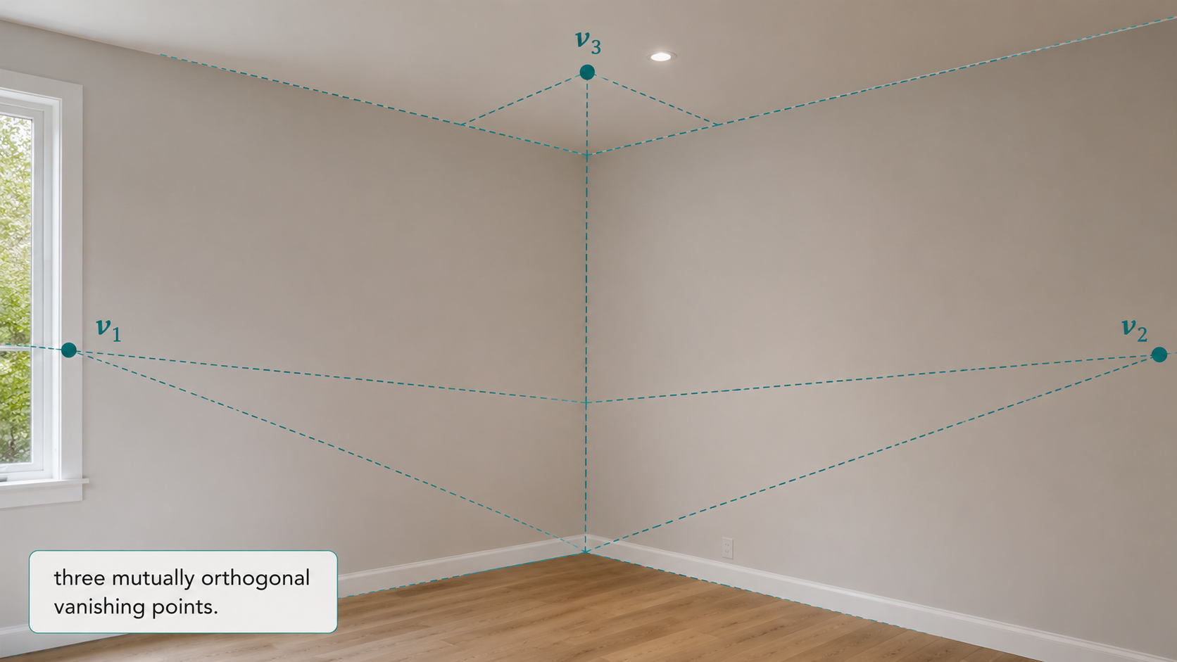
One pair of perpendicular vanishing points gives 1 constraint. Two pairs give 2 constraints. Three mutually perpendicular pairs — which correspond to three orthogonal planes, like the three faces of a room corner — give 3 constraints:

\[\mathbf{v}_1^T \omega \mathbf{v}_2 = 0, \quad \mathbf{v}_1^T \omega \mathbf{v}_3 = 0, \quad \mathbf{v}_2^T \omega \mathbf{v}_3 = 0\]

That’s still only 3 constraints for 5 unknowns. We’re short by 2. Here is where a common and practically reasonable assumption saves us: if we assume the camera has zero skew (the pixels are rectangular, not parallelogram-shaped) and square pixels (equal horizontal and vertical pixel density), then $\omega$ takes the simplified form:

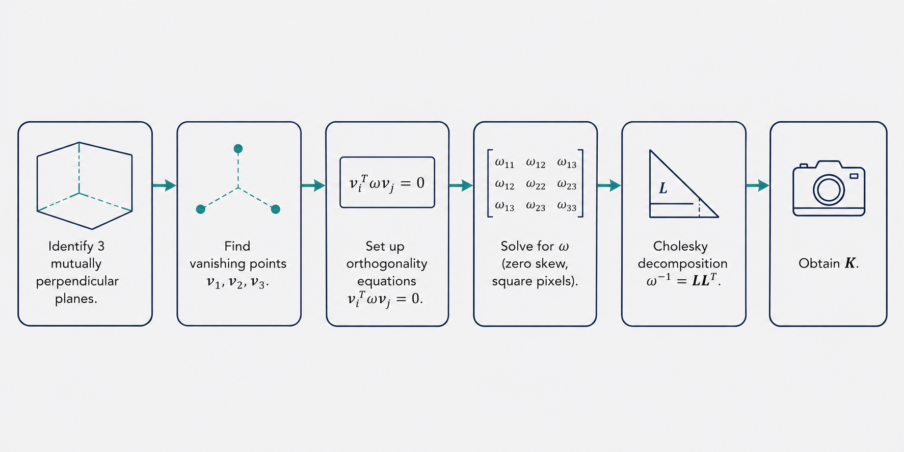
\[\omega = \begin{pmatrix} \omega_1 & 0 & \omega_4 \\ 0 & \omega_1 & \omega_5 \\ \omega_4 & \omega_5 & \omega_6 \end{pmatrix}\]

This form has only 4 distinct parameters. Since $\omega$ is determined only up to scale, we effectively have 3 free parameters. The three orthogonality constraints from three mutually perpendicular vanishing points are exactly enough to solve for this $\omega$.

From $\omega$ to $K$: Cholesky Decomposition

Once $\omega$ is determined, recovering $K$ is a standard numerical procedure. Recall that $\omega = (KK^T)^{-1}$, which means $\omega^{-1} = KK^T$. This says that $\omega^{-1}$ is a positive-definite symmetric matrix with a specific factorization. The Cholesky decomposition finds the unique lower-triangular matrix $L$ such that $\omega^{-1} = LL^T$. Since $K$ must be upper-triangular (by convention in camera models), we identify $K = L^T$.

The entire pipeline thus looks like this: identify three mutually perpendicular planes in the image → find their vanishing points → set up the three orthogonality equations → solve for $\omega$ → apply Cholesky decomposition → obtain $K$. A single photograph, with no calibration target, has yielded the full intrinsic calibration of the camera.

What Comes Next: Recovering 3D Geometry

With $K$ in hand, the door to 3D reconstruction swings open. For any plane visible in the image, we can:

Find the horizon line of that plane (from the vanishing points of lines in the plane).
Recover the plane’s 3D normal direction via $\mathbf{n} = K^T \ell_{\text{horiz}}$.
Compute angles between planes using their horizon lines and $\omega^{-1}$.
Recover the 3D directions of any family of parallel lines using $\mathbf{d} = K^{-1}\mathbf{v} / |K^{-1}\mathbf{v}|$.

What began as a flat photograph has been transformed, through the mathematics of projective geometry, into a partial but rich 3D model of the scene.

Part 5: Conceptual Synthesis — What the Mathematics Tells Us

It is worth pausing to appreciate the conceptual arc of what we have covered.

The projective transformation is the right mathematical model for what a camera does. It destroys some geometric information — most notably, parallelism — but it preserves other things: the cross-ratio of four collinear points, collinearity itself, and crucially, the directions of parallel lines (in the form of vanishing points). The camera does not destroy information randomly; it transforms it in a systematic, invertible (given enough constraints) way.

The line at infinity in 2D, and the plane at infinity in 3D, are not mystical constructs but practical tools. The plane at infinity in 3D — defined by the vector $(0, 0, 0, 1)^T$ in homogeneous coordinates — is the “home” of all directions in 3D space. When the camera projects the scene, it maps this plane at infinity to a finite region of the image, and the structure of that mapping (encoded by $\omega$) tells us everything about how the camera distorts angles. Recovering $\omega$ is equivalent to understanding how the camera has “compressed” the plane at infinity into the image.

The assumption of zero skew and square pixels is worth reflecting on. These are not exotic constraints — they are satisfied by virtually every modern digital camera. By incorporating this common-sense knowledge about camera construction, we close the gap between the geometric constraints available from the scene and the number of unknowns in the camera model. Prior knowledge about the camera compensates for what the scene cannot tell us alone.

There is also a beautiful symmetry in the angle formulas. The same matrix $\omega = (KK^T)^{-1}$ appears in both the line-direction angle formula and the plane-normal angle formula (using $\omega^{-1}$ in the latter). This is not a coincidence: $\omega$ is precisely the metric tensor of the image plane that corrects for the projective distortion of the camera. It is the Rosetta Stone that translates between image measurements and 3D angular measurements.

Conclusion: One Image, a World of Information

The ideas explored here collectively answer a question that might initially seem impossible: what can one photograph tell us about the 3D world that produced it? As we have seen, the answer is “quite a lot” — provided we know how to listen.

The hierarchy of transformations — from rigid isometries to similarities, affinities, and finally projective transformations — establishes the precise way in which perspective imaging distorts the world. The concept of points and lines at infinity provides a mathematically coherent way to talk about direction and parallelism even in the projected image. Vanishing points are the image of these ideal points, and they encode the 3D directions of parallel lines. Horizon lines encode the orientation of planes. And the matrix $\omega$, derived from the camera’s intrinsic parameters, is the key that unlocks angular measurements from image coordinates alone.

The culminating result — that three mutually perpendicular vanishing points from a single photograph, combined with the mild assumption of a well-behaved camera, are sufficient to calibrate the camera — is a testament to how much structure is hidden inside an ordinary image. Every photograph of an architectural scene, a room interior, or a city street is simultaneously a record of the visual scene and a rich geometric document waiting to be decoded.

This is the spirit of single view metrology: not merely asking what a photograph shows, but asking what the geometry of the photograph reveals about the world that made it.

This article is based on CS231A Course Notes 2: Single View Metrology, by Kenji Hata and Silvio Savarese, Stanford University.

Single View Metrology