Seeing in 3D: How Computers Reconstruct the World from Flat Images

Seeing in 3D: How Computers Reconstruct the World from Flat Images

A deep dive into triangulation, stereo vision, and structure from motion — the algorithms that let machines perceive depth.

Introduction: The Depth Illusion

Close one eye and reach for a nearby object. You will likely miss it — or at least feel strangely uncertain about how far away it is. Your visual system suddenly loses something it normally takes for granted: depth. The brain reconstructs a 3D world by comparing the slightly different images received by each eye, a process called stereopsis. The difference in position of an object between the two eyes — called disparity — encodes how far away the object is.

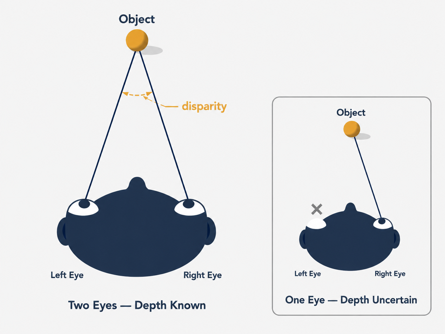
Cameras, unlike eyes, capture flat 2D images. A single photograph flattens the entire richness of a three-dimensional scene into a plane, discarding depth information entirely. A point appearing in a photograph could be close and small, or far away and large — the image alone cannot tell you which. This is the fundamental challenge of 3D computer vision: recovering the depth, structure, and geometry of a world that has been projected down onto a flat sensor.

Yet this is exactly what modern systems do, with remarkable success. The GPS in your phone reconstructs satellite geometry to locate you on Earth. Autonomous vehicles build 3D maps in real time from cameras. Photogrammetry software turns a handful of vacation photos into a detailed 3D model of a cathedral. Augmented reality apps overlay digital objects onto the physical world with precise spatial alignment. All of these depend on the same core algorithmic ideas: triangulation, stereo reconstruction, and structure from motion (SfM).

In this article, we will build up these ideas from first principles — not just explaining what the algorithms do, but why they work, what makes them tricky in practice, and how the mathematics captures the geometry of vision.

Part 1: Triangulation — Finding Where Rays Meet

The Core Idea

Here is the simplest version of the 3D reconstruction problem. You have two cameras, both looking at the same scene. You can see the same physical point $P$ in both images — at position $p$ in the first image and $p’$ in the second. You know everything about both cameras: their intrinsic parameters (focal length, principal point, pixel scaling) encoded in matrices $K$ and $K’$, and their relative rotation $R$ and translation $T$ with respect to each other.

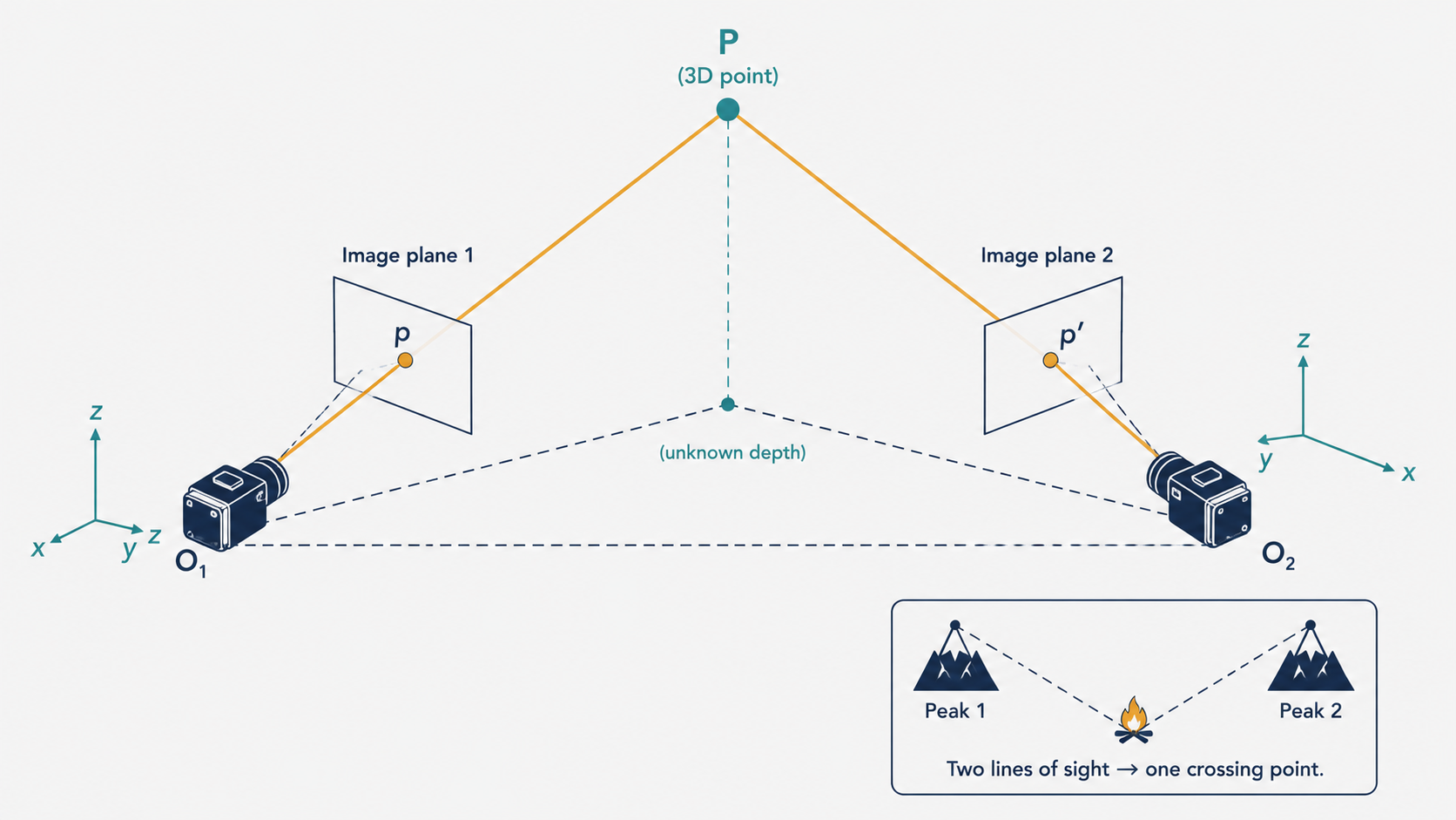
Given all of this, where is $P$ in 3D space?

The answer seems almost obvious once you draw the picture. Each observed image point, combined with the camera center, defines a ray in 3D space — a line emanating from the camera through the image point and extending into the scene. The first camera gives you ray $\ell$, the second gives you ray $\ell’$. The 3D point $P$ must lie on both rays simultaneously, so $P$ is simply the intersection of $\ell$ and $\ell’$. This is the essence of triangulation.

Think of it like two search parties trying to locate a missing hiker from different mountain peaks. Each party can see the hiker’s fire and knows what direction it lies in — but not the distance. If both parties know exactly where they are standing and which direction they are looking, they can draw two lines on a map and find where the lines cross. That crossing point is where the fire must be.

Why Perfect Intersection Rarely Exists

In theory, the two rays $\ell$ and $\ell’$ must intersect — after all, they both pass through the same physical point $P$. In practice, they almost never intersect cleanly.

The culprit is noise. The pixel locations $p$ and $p’$ are measured with some error due to sensor noise, lens distortion, and quantization effects. The camera calibration parameters $K$, $K’$, $R$, $T$ are also estimated from data, and thus carry their own errors. When you compute the rays based on imprecise inputs, the rays end up slightly skewed — passing near each other but not through a common point. In 3D space, two lines that are not parallel and do not intersect are called skew lines, and skew lines are the rule rather than the exception in real-world triangulation.

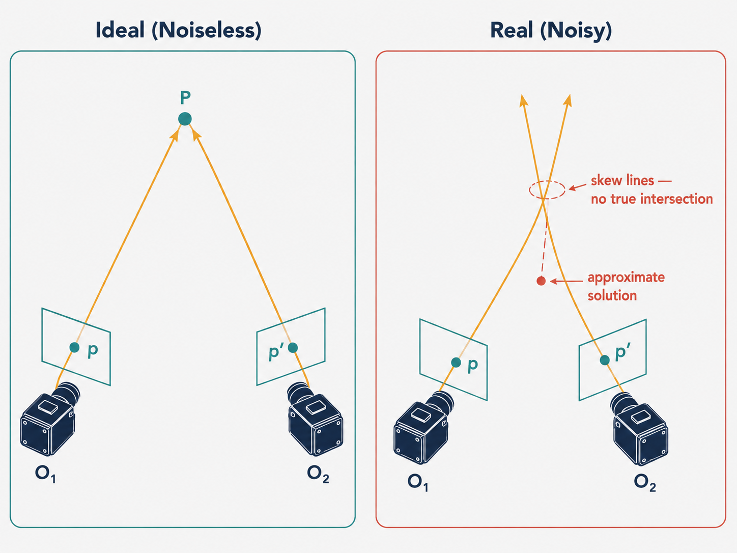
This means we cannot simply find an exact intersection. Instead, we need to find the best approximate answer. There are two main strategies for doing this, each with different trade-offs.

Strategy 1: The Linear Method (DLT)

The first approach reformulates triangulation as a system of linear equations. Starting from the projection equation $p = MP$ (where $M$ is the $3 \times 4$ camera matrix), we use a key algebraic observation: since $p$ and $MP$ represent the same point in homogeneous coordinates, their cross product is zero:

\[p \times (MP) = 0\]

Expanding this cross product gives three scalar equations:

$x(M_3 P) - (M_1 P) = 0$ $y(M_3 P) - (M_2 P) = 0$ $x(M_2 P) - y(M_1 P) = 0$

where $M_i$ denotes the $i$-th row of the camera matrix $M$, and $(x, y, 1)$ are the homogeneous coordinates of the image point $p$. Each observed correspondence contributes a pair of independent constraints (the third equation is redundant). Stacking the constraints from both cameras, we get a homogeneous linear system:

\[A P = 0, \quad \text{where} \quad A = \begin{pmatrix} xM_3 - M_1 \\ yM_3 - M_2 \\ x'M'_3 - M'_1 \\ y'M'_3 - M'_2 \end{pmatrix}\]

This is a standard Singular Value Decomposition (SVD) problem. We find the vector $P$ that minimizes $|AP|$ subject to $|P| = 1$, which is simply the right singular vector of $A$ corresponding to its smallest singular value.

One elegant property of this formulation is that it generalizes seamlessly to more than two cameras. If you add a third camera with its own observation, you simply append two more rows to the matrix $A$. The SVD solution naturally incorporates all available observations.

However, the linear method has a critical flaw: it is not invariant under projective transformations. If we apply a projective transformation $H$ to the camera matrices (replacing $M$ with $MH^{-1}$), the system matrix becomes $AH^{-1}$, and the old solution $P$ now corresponds to $HP$ in the new coordinate system. But the SVD imposes the constraint $|P| = 1$, which is not preserved under a projective transformation $H$. This means that in projective reconstruction settings, the linear method does not give the geometrically optimal answer. It is a convenient starting point, but not the final word.

Strategy 2: The Nonlinear Method (Minimizing Reprojection Error)

A more principled approach frames triangulation as a minimization problem. Rather than asking “where do the rays intersect?” we ask: “what 3D point, when projected into both cameras, best explains the observed image points?”

Formally, we want to find a 3D point $\hat{P}$ that minimizes the total reprojection error:

\[\min_{\hat{P}} \; \|M\hat{P} - p\|^2 + \|M'\hat{P} - p'\|^2\]

The term $|M\hat{P} - p|^2$ measures the pixel distance between where $\hat{P}$ actually projects in image 1 (at $M\hat{P}$) and where we observed it (at $p$). This is the reprojection error for image 1. The full objective sums these errors across all images:

\[\min_{\hat{P}} \; \sum_i \|M_i \hat{P} - p_i\|^2\]

Intuitively, this says: find the 3D point whose “shadow” in each camera is as close as possible to the actual observed shadow. This is geometrically meaningful and robust to noise in a way that the linear method is not.

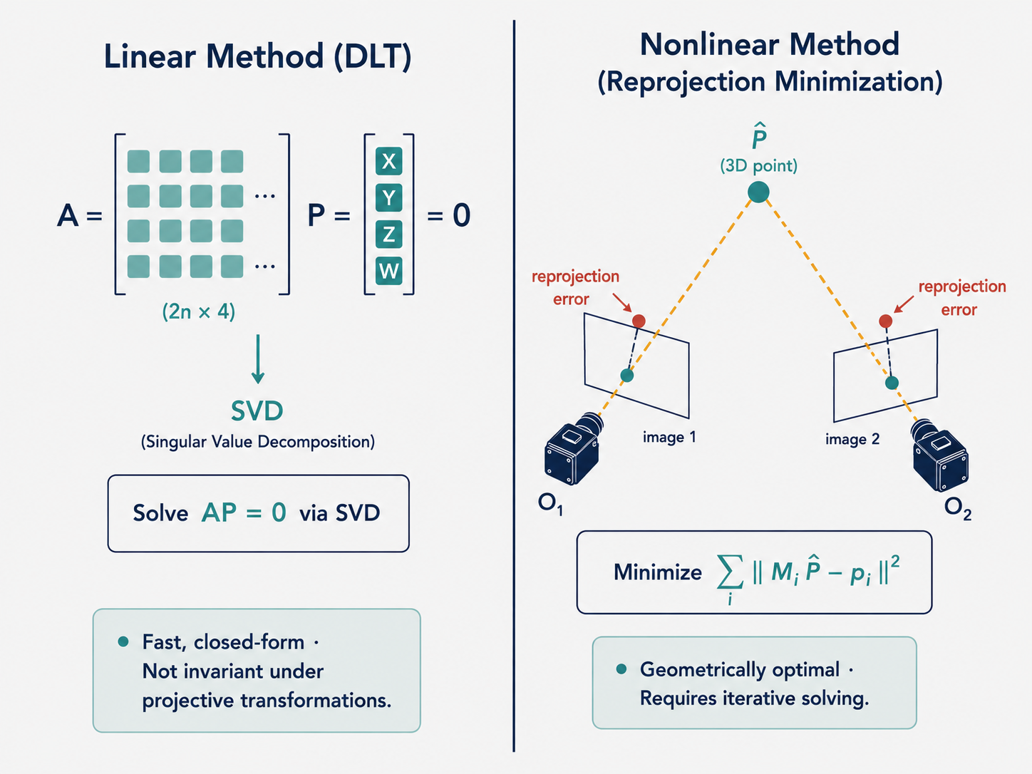
The challenge is that this is a nonlinear optimization problem. The camera projection involves a division by the homogeneous coordinate (the perspective divide), which introduces nonlinearity. We cannot solve it with a single matrix operation.

The Gauss-Newton Algorithm: Linearizing the Nonlinear

The standard approach to nonlinear least squares problems like this is the Gauss-Newton algorithm, a powerful iterative method. The key insight is beautiful: even though the overall problem is nonlinear, near our current estimate, the function looks approximately linear.

Here is the idea. Suppose we have a current estimate $\hat{P}$ of the 3D point (which we can initialize with the linear method). We want to find a small correction $\delta P$ such that $\hat{P} + \delta P$ gives a lower reprojection error. We linearize the residual function $e(\hat{P})$ using a first-order Taylor expansion:

\[e(\hat{P} + \delta P) \approx e(\hat{P}) + \frac{\partial e}{\partial P} \delta P\]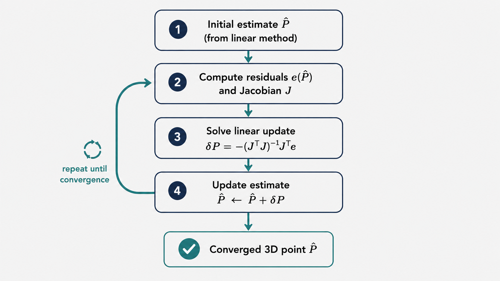

Substituting this into the minimization, the problem becomes:

\[\min_{\delta P} \; \left\| \frac{\partial e}{\partial P} \delta P - (-e(\hat{P})) \right\|^2\]

This is now a standard linear least squares problem! The solution is:

\[\delta P = -(J^T J)^{-1} J^T e\]

where $J = \frac{\partial e}{\partial P}$ is the Jacobian matrix of the residuals with respect to the 3D point coordinates, and $e$ is the stacked vector of residuals from all cameras.

In the simplest two-camera case ($N = 2$), each residual $e_i$ is a $2 \times 1$ vector (one error per image dimension), so the total residual vector $e$ is $4 \times 1$ and the Jacobian $J$ is $4 \times 3$. We repeatedly compute this update, re-evaluate the Jacobian at the new estimate, and continue until convergence.

One important caveat: since the Gauss-Newton method relies on a local linear approximation, it does not guarantee convergence to the global minimum. If the initial estimate is poor, the algorithm may diverge or settle in a bad local minimum. This is why we always warm-start it with the linear estimate — even a rough linear solution gives Gauss-Newton a good enough starting point to converge reliably.

Part 2: Structure from Motion — Solving the Full Puzzle

From Two Views to Many

Triangulation solves a specific problem: given camera positions, find point positions. But what if we do not know where the cameras are? What if we have a large collection of photos taken from arbitrary positions, and we want to recover both the 3D structure of the scene and the camera positions simultaneously?

This is the structure from motion (SfM) problem, and it is significantly more challenging — and more powerful.

Think of it like archaeology. An archaeologist discovers a collection of paintings in a cave, each showing the same landscape from a slightly different angle. By studying the overlapping features across paintings, the archaeologist can deduce both the layout of the original landscape (the structure) and where each painter was standing (the motion). SfM does exactly this, but with mathematical precision.

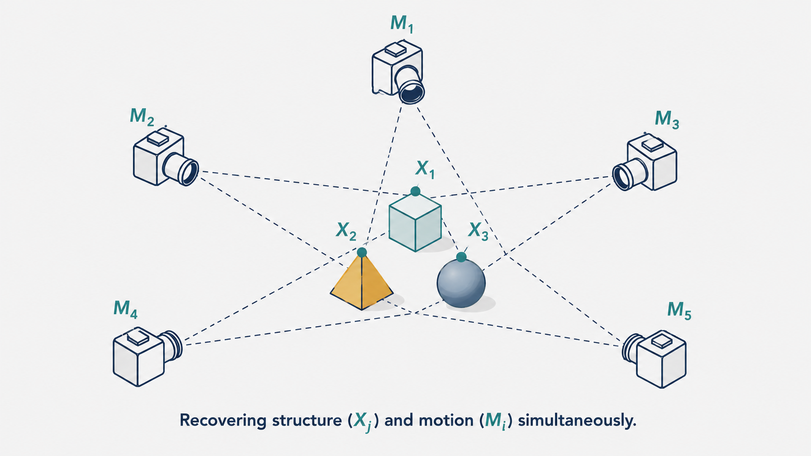
Formally, suppose we have $m$ cameras with projection matrices $M_i$ and $n$ 3D points $X_j$ in the scene. Each point $X_j$ appears in camera $i$ at image location $x_{ij}$. The goal of SfM is to recover:

All $n$ points $X_j$ — the structure of the scene.
All $m$ projection matrices $M_i$ — the motion of the cameras.

from the observed image locations $x_{ij}$.

Part 3: Affine Structure from Motion

A Simpler Camera Model to Build Intuition

Before tackling the full projective case, we start with a simplified camera model called the affine (or weak perspective) camera. In the standard perspective camera, the projection divides by depth, creating a nonlinear transformation. The affine camera drops this division, approximating the scene as if all objects are at roughly the same depth.

In the full perspective model, the camera matrix has the form:

\[M = \begin{pmatrix} A & b \\ v & 1 \end{pmatrix}\]

where $v$ is a non-zero row vector capturing the perspective effect. In the affine model, we set $v = 0$. This makes the homogeneous coordinate of any projected point equal to 1, so the projection simplifies to a pure linear mapping:

\[\begin{pmatrix} u \\ v \end{pmatrix} = AX + b\]

where $A$ is a $2 \times 3$ matrix and $b$ is a $2 \times 1$ translation vector. The transformation is now entirely linear — no division by depth. While this sacrifices some accuracy for scenes with significant depth variation, it makes the mathematics tractable and provides valuable intuition for the general case.

Counting Unknowns and Equations

Let us get a feel for the scale of the problem. With $m$ affine cameras, each described by an $A_i$ (6 parameters) and $b_i$ (2 parameters), we have $8m$ camera unknowns. With $n$ 3D points, each with 3 coordinates, we have $3n$ structure unknowns. The total unknowns: $8m + 3n$.

Each observation $x_{ij}$ provides 2 equations (the $x$ and $y$ image coordinates). With $mn$ observations, we have $2mn$ equations. For the system to be solvable, we need $2mn \geq 8m + 3n$. As a sanity check: with $m = 2$ cameras, we need at least $n = 16$ point correspondences.

The Tomasi-Kanade Factorization Method

The elegant solution to the affine SfM problem was proposed by Tomasi and Kanade in a landmark 1992 paper. Their key insight was to reformulate the problem as a matrix factorization — specifically, writing all observations as a matrix product that can be decomposed using SVD.

Step 1: Data Centering

The first step is to center the data. For each camera $i$, subtract the centroid $\bar{x}_i$ of all observed image points:

\[\hat{x}_{ij} = x_{ij} - \bar{x}_i = x_{ij} - \frac{1}{n} \sum_{j=1}^{n} x_{ij}\]

Why center? Because the affine projection is $x_{ij} = A_i X_j + b_i$. When we subtract the mean image coordinates, the translation $b_i$ vanishes. This is because the mean of $A_i X_j + b_i$ over all $j$ is $A_i \bar{X} + b_i$, and after centering:

\[\hat{x}_{ij} = x_{ij} - \bar{x}_i = A_i X_j + b_i - (A_i \bar{X} + b_i) = A_i (X_j - \bar{X}) = A_i \hat{X}_j\]

The translation term has completely disappeared. The centered image coordinates and centered 3D coordinates are now related by the simple linear relationship $\hat{x}_{ij} = A_i \hat{X}_j$.

Think of centering as moving your coordinate system’s origin to the “average” location of all the points. Once you are working relative to this center, translations no longer matter — everything is pure rotation and scaling.

Step 2: Building the Measurement Matrix

Now that we have the relationship $\hat{x}_{ij} = A_i \hat{X}_j$, we can assemble all observations into a single large matrix $D$:

\[D = \begin{pmatrix} \hat{x}_{11} & \hat{x}_{12} & \cdots & \hat{x}_{1n} \\ \hat{x}_{21} & \hat{x}_{22} & \cdots & \hat{x}_{2n} \\ \vdots & & & \vdots \\ \hat{x}_{m1} & \hat{x}_{m2} & \cdots & \hat{x}_{mn} \end{pmatrix}\]

Each entry $\hat{x}_{ij}$ is a $2 \times 1$ vector, so $D$ is a $2m \times n$ matrix. Crucially, this matrix can be written as a product:

\[D = \underbrace{\begin{pmatrix} A_1 \\ A_2 \\ \vdots \\ A_m \end{pmatrix}}_{\text{motion matrix } \mathcal{M}} \underbrace{\begin{pmatrix} \hat{X}_1 & \hat{X}_2 & \cdots & \hat{X}_n \end{pmatrix}}_{\text{structure matrix } \mathcal{S}}\]

The motion matrix $\mathcal{M}$ is $2m \times 3$ and the structure matrix $\mathcal{S}$ is $3 \times n$. Because $D$ is the product of a $2m \times 3$ matrix and a $3 \times n$ matrix, its rank is at most 3. This is the mathematical key that unlocks the factorization.

Step 3: SVD Factorization

Given that $\text{rank}(D) = 3$, we can apply SVD and truncate to the top 3 components:

\[D = U \Sigma V^T \approx U_3 \Sigma_3 V_3^T\]

where $\Sigma_3 = \text{diag}(\sigma_1, \sigma_2, \sigma_3)$ contains only the three largest singular values, and $U_3$, $V_3$ contain the corresponding three left and right singular vectors.

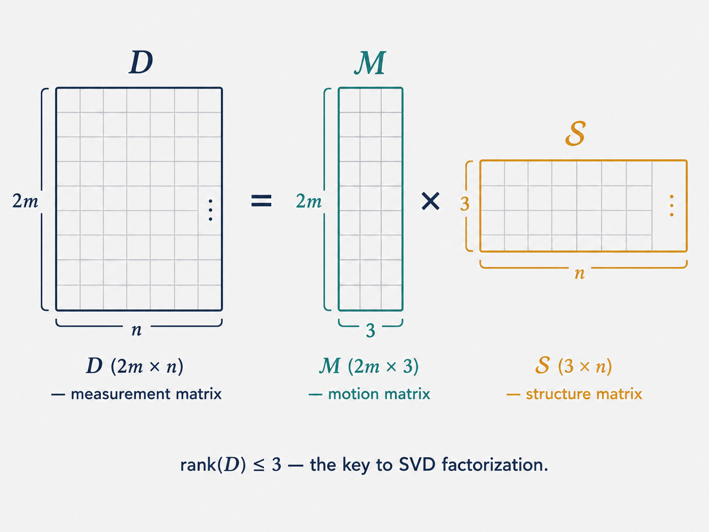
The key step is to associate this decomposition with the motion and structure matrices. Tomasi and Kanade showed that a robust and geometrically meaningful factorization is:

\[\mathcal{M} = U_3 \sqrt{\Sigma_3}, \quad \mathcal{S} = \sqrt{\Sigma_3} V_3^T\]

The choice is not unique — any invertible $3 \times 3$ matrix $A$ could be inserted as $D = (\mathcal{M} A)(A^{-1} \mathcal{S})$ and the product would still be $D$. This is the affine ambiguity, which we will discuss shortly. But distributing the singular values symmetrically as $\sqrt{\Sigma_3}$ gives a stable, balanced decomposition.

In practice, measurement noise makes $\text{rank}(D) > 3$. But the truncated SVD still gives the best rank-3 approximation of $D$ in the Frobenius norm sense — the closest rank-3 matrix to the noisy observations. This is a beautiful property of SVD that makes the method robust.

Part 4: Ambiguity in Reconstruction

The Unavoidable Unknowns

Before moving on, we need to confront an important conceptual issue: even with a perfect algorithm and noiseless data, some things about a 3D scene are fundamentally unrecoverable from images alone.

The most obvious one: absolute scale. If you see a house in a photograph, you cannot tell if it is a full-sized building 100 meters away or a dollhouse model 1 meter away. The images look identical. Without additional information — a ruler in the scene, knowledge of the size of some object, GPS coordinates — scale is lost.

More formally, there are different levels of reconstruction ambiguity:

Affine ambiguity arises in the affine SfM setting. Any invertible $3 \times 3$ matrix $A$ could be inserted into the factorization $D = \mathcal{M} \mathcal{S} = (\mathcal{M}A)(A^{-1}\mathcal{S})$ without changing the observations. This means the camera matrices and 3D points are only determined up to an affine transformation. Affine transformations preserve parallelism but can distort angles and distances.

Similarity ambiguity is a milder version. A reconstruction has only similarity ambiguity if it is correct up to a rigid transformation (rotation, translation) plus uniform scaling. This is known as a metric reconstruction. Even with fully calibrated cameras, similarity ambiguity remains — you know the shape and proportions of the scene perfectly, but not its absolute size or orientation relative to some external coordinate system.

Projective ambiguity is the most severe. In the general projective SfM case, the reconstruction is only defined up to a $4 \times 4$ projective transformation, which can distort the scene significantly.

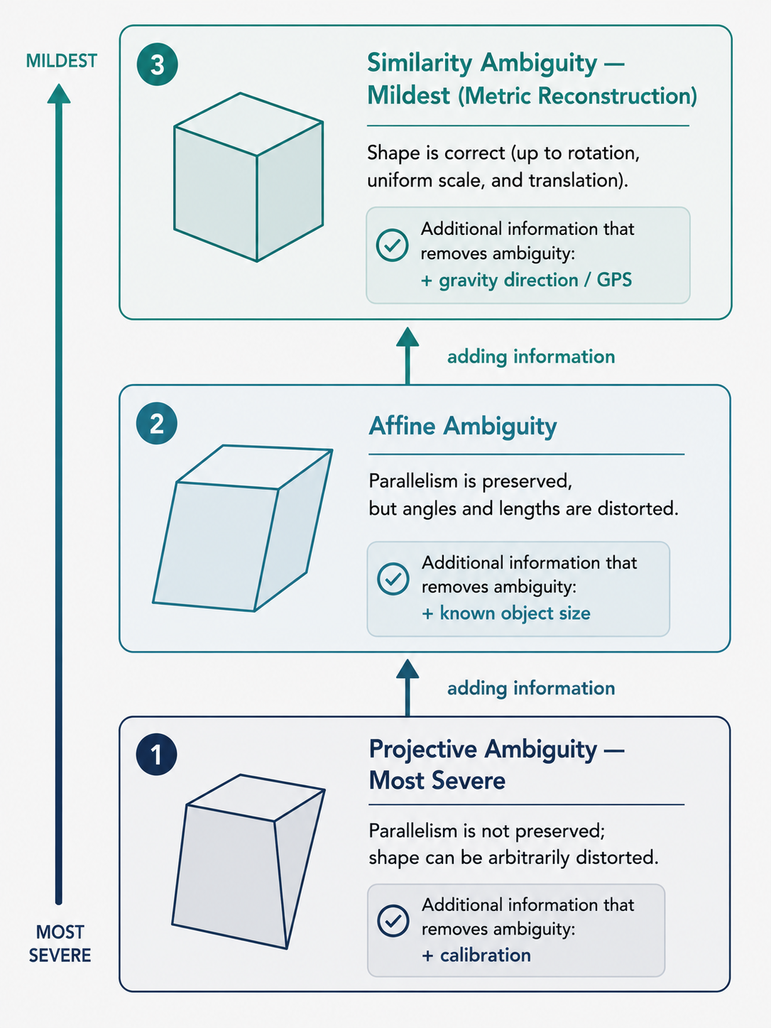
Each level of ambiguity can be removed by adding more constraints. Knowing the height of an object removes scale ambiguity. Knowing the calibration of the camera removes projective ambiguity. Knowing the direction of gravity removes rotation ambiguity. The hierarchy of ambiguities reflects a hierarchy of what information images can and cannot provide.

Part 5: Perspective Structure from Motion

The General (Projective) Case

Real cameras are perspective cameras, not affine ones. The full projective camera matrix has 11 degrees of freedom (a $3 \times 4$ matrix defined up to scale):

\[M_i = \begin{pmatrix} a_{11} & a_{12} & a_{13} & b_1 \\ a_{21} & a_{22} & a_{23} & b_2 \\ a_{31} & a_{32} & a_{33} & 1 \end{pmatrix}\]

With $m$ cameras and $n$ 3D points, and accounting for the projective ambiguity (a $4 \times 4$ matrix up to scale, meaning 15 free parameters), we have $11m + 3n - 15$ unknowns and $2mn$ equations. Plugging in small values tells us: with just 3 cameras, we need roughly 5 or more point correspondences to have a determined system.

The structure and motion can only be recovered up to a projective transformation — a $4 \times 4$ invertible matrix $H$. This is because applying $H$ to the 3D points and $H^{-1}$ to the camera matrices leaves all image projections unchanged.

The Algebraic Approach: Using the Fundamental Matrix

One elegant method for solving the two-camera projective SfM problem uses the fundamental matrix $F$, which encodes the epipolar geometry between two views. The key insight is to use $F$ to directly compute the camera matrices.

Since camera matrices are only determined up to a projective transformation $H$, we can always choose $H$ such that the first camera has a canonical form:

\[\tilde{M}_1 = [I \mid 0], \quad \tilde{M}_2 = [A \mid b]\]

The first camera is placed at the origin, looking forward — this is our reference frame. The second camera’s matrix encodes the relative motion between the cameras.

Now, how do we find $A$ and $b$? A beautiful algebraic derivation shows that if we define $F = [b]\times A$ (where $[b]\times$ denotes the skew-symmetric cross-product matrix of vector $b$), then the constraint $p’^T F p = 0$ is satisfied — exactly the fundamental matrix constraint. This means:

$b$ is the epipole — the projection of the first camera center into the second image. It satisfies $F^T b = 0$ and can be computed as the null vector of $F^T$ via SVD.

Once $b$ is known, we can recover $A$:

\[A = -[b]_\times F\]

which can be verified by substituting into $F = [b]_\times A$:

\[[b]_\times A = -[b]_\times [b]_\times F = (bb^T - |b|^2 I)F = bb^T F + F = F\]

using the identity $[b]\times [b]\times = bb^T -

^2 I$ and the fact that $Fb = 0$.

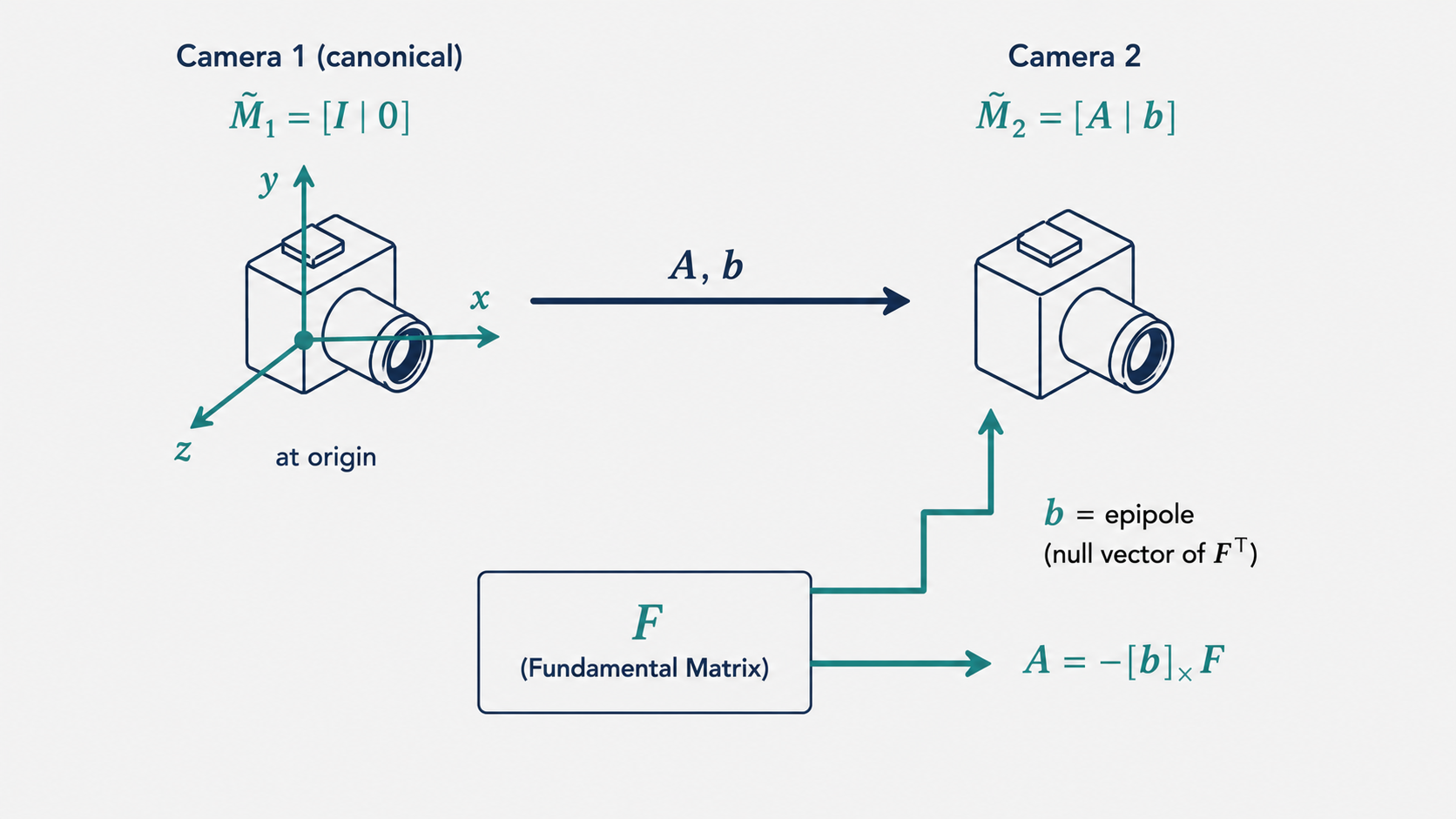
The final camera matrices are:

\[\tilde{M}_1 = [I \mid 0], \quad \tilde{M}_2 = [-[e]_\times F \mid e]\]

where $e$ is the epipole (second column, i.e., $b$). This is a complete, closed-form solution for the camera matrices given $F$.

Using the Essential Matrix for Calibrated Cameras

When the cameras are calibrated (the intrinsic matrices $K$ and $K’$ are known), we can do better. The Essential matrix $E$ is the fundamental matrix in normalized (calibrated) image coordinates:

\[E = K^T F K\]

Because $E$ works with calibrated coordinates, it strips away the intrinsic parameters and encodes only the extrinsic relationship between cameras: the rotation $R$ and translation $t$. This means $E$ has only 5 degrees of freedom (3 for rotation, 3 for translation, minus 1 for scale).

The Essential matrix can be written as:

\[E = [t]_\times R\]

where $[t]_\times$ is the skew-symmetric matrix of the translation vector. Factoring $E$ into $R$ and $t$ is a non-trivial decomposition. The derivation relies on two auxiliary matrices:

\[W = \begin{pmatrix} 0 & -1 & 0 \\ 1 & 0 & 0 \\ 0 & 0 & 1 \end{pmatrix}, \quad Z = \begin{pmatrix} 0 & 1 & 0 \\ -1 & 0 & 0 \\ 0 & 0 & 0 \end{pmatrix}\]

A key property: $Z = \text{diag}(1,1,0) W$ up to sign, and $ZW = ZW^T = \text{diag}(1,1,0)$ up to sign.

Since $[t]_\times$ is skew-symmetric, it can be decomposed using its Jordan form as:

\[[t]_\times = U Z U^T\]

for some orthogonal matrix $U$. Substituting this into $E = [t]_\times R$:

\[E = U \, \text{diag}(1,1,0) \, (W U^T R)\]

Comparing with the SVD $E = U \Sigma V^T$ (where $\Sigma = \text{diag}(1,1,0)$), the factorization yields:

$R = U W V^T \quad \text{or} \quad R = U W^T V^T$ $t = \pm U \begin{pmatrix} 0 \\ 0 \\ 1 \end{pmatrix} = \pm u_3$

where $u_3$ is the third column of $U$.

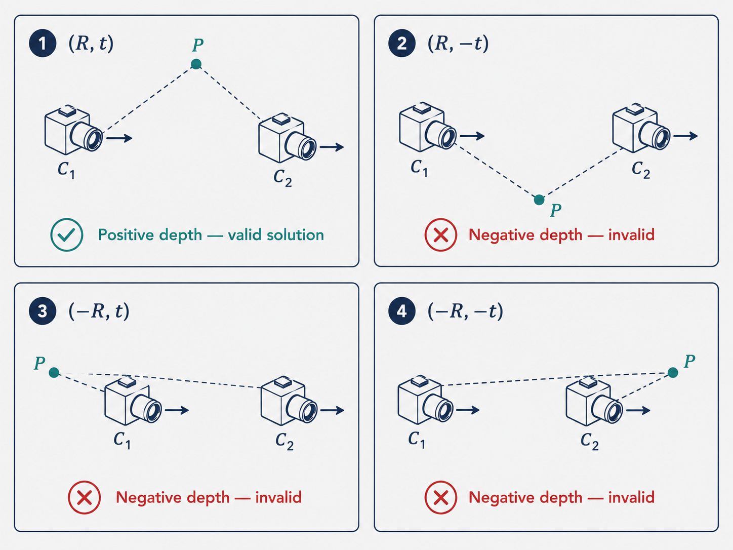
This gives four candidate solutions: two for $R$ and two for $t$. In practice, only one of these four corresponds to the physically meaningful case where the reconstructed scene point lies in front of both cameras (positive depth). We resolve the ambiguity by triangulating one (or a few) test points and checking which configuration produces positive depths in both camera coordinate systems. The correct $(R, t)$ pair is unambiguous in practice.

Part 6: Bundle Adjustment — The Final Polish

The Limitations of Pairwise Methods

Both the factorization approach and the algebraic approach have important limitations. The factorization method requires all points to be visible in every image — a requirement that fails whenever objects are occluded or cameras are too far apart for features to match. The algebraic approach handles pairs of cameras, but chaining these pairwise solutions can accumulate errors: inaccuracies in the first pair compound into larger errors as more cameras are added.

What we really want is a method that considers all cameras and all points simultaneously, minimizing a globally consistent objective across the entire dataset.

Bundle Adjustment: Global Optimization

Bundle adjustment is that method. It takes as input an initial estimate of all camera matrices $M_i$ and all 3D points $X_j$ (obtained from one of the preceding methods), and jointly refines all of them by minimizing the total reprojection error across all visible observations:

\[\min_{\{M_i\}, \{X_j\}} \; \sum_{i,j \in \mathcal{V}} \|M_i X_j - x_{ij}\|^2\]

where $\mathcal{V}$ is the set of $(i, j)$ pairs for which point $j$ is visible in camera $i$.

The name “bundle adjustment” comes from the geometric picture: each camera emits a bundle of rays toward the observed points. The optimization adjusts both the camera positions and the point positions so that these bundles are as consistent as possible across all views.

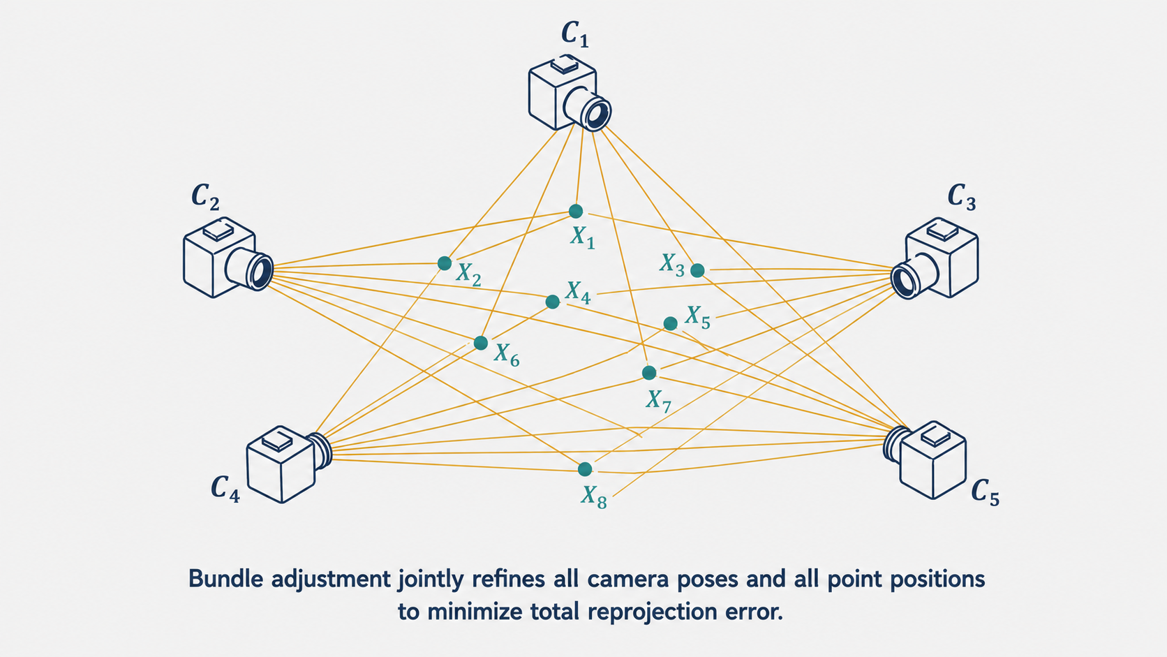
This is a large nonlinear least squares problem, typically solved using the Gauss-Newton or Levenberg-Marquardt algorithm. The Levenberg-Marquardt algorithm is a hybrid between Gauss-Newton and gradient descent — it is more conservative when the current estimate is far from the solution, and more aggressive (like Gauss-Newton) when near convergence. This makes it much more robust to poor initializations.

The Role of Bundle Adjustment in a Full SfM Pipeline

Bundle adjustment is almost never run from scratch. The optimization landscape has many local minima, and converging to a good solution requires a reasonable starting point. The typical SfM pipeline therefore proceeds in stages:

Feature extraction and matching: Find distinctive keypoints (like SIFT or ORB features) in all images and match them across pairs of images. These matches provide the point correspondences $x_{ij}$.
Initial reconstruction: Use the algebraic approach (via the fundamental or essential matrix) on a well-chosen initial pair of cameras to get a rough initial reconstruction of some 3D points and two camera poses.
Incremental expansion: Add cameras one by one. For each new camera, use the already-reconstructed 3D points to estimate the new camera’s pose via the PnP (Perspective-n-Point) algorithm, then triangulate new points visible from the new camera.
Bundle adjustment: After adding each new camera (or after adding a batch of cameras), run bundle adjustment to “tighten” the reconstruction and prevent accumulated errors from growing.

The factorization and algebraic methods provide good initializations. Bundle adjustment provides the final, high-accuracy polish. Together, they form a robust pipeline for reconstructing 3D scenes from unstructured photo collections.

Trade-offs and Practical Considerations

Bundle adjustment has remarkable strengths. It handles arbitrary numbers of cameras and arbitrary patterns of point visibility. It leverages all the data simultaneously, so errors in individual measurements are averaged out. And it produces the statistically optimal estimate under Gaussian noise assumptions.

Its main limitation is computational cost. The number of unknowns grows with both the number of cameras ($11m$) and the number of points ($3n$), and the Jacobian matrix can be enormous for large reconstructions. Fortunately, the problem has a special sparse structure — each point only interacts with the cameras that can see it — and modern bundle adjustment solvers (like Ceres Solver or g2o) exploit this sparsity to solve problems with thousands of cameras and millions of points efficiently.

The other limitation is sensitivity to initialization. Bundle adjustment is a local optimization method and can get trapped in local minima. This is why the preceding pairwise methods are so important — they provide a good enough starting point that the final optimization converges to the right solution.

Putting It All Together: A Modern SfM Pipeline

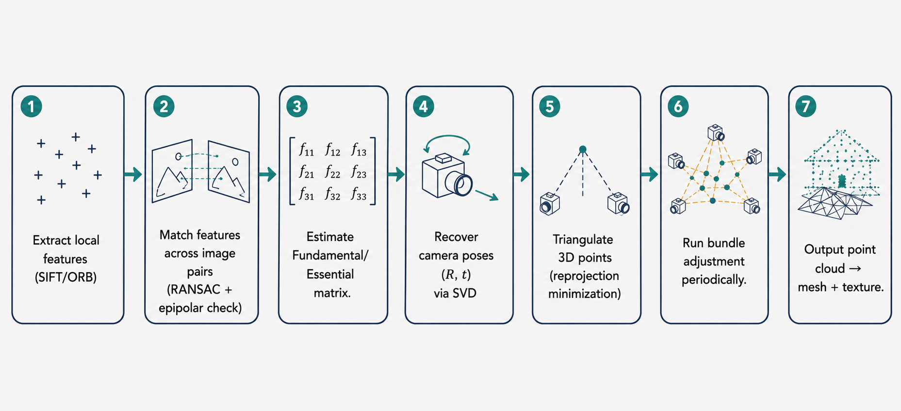
To see how all these pieces fit, let us trace through a concrete example: you take 50 photographs of a building from different angles, upload them to a photogrammetry tool, and get back a 3D model. Here is what is happening under the hood:

The software first extracts local features from every image — small, distinctive patches around corners, edges, and texture boundaries. These features are described by high-dimensional vectors (SIFT descriptors, for instance) that are designed to be stable across changes in scale, rotation, and lighting.

Next, pairs of images with overlapping content are identified, and feature matches are established. A robust fitting algorithm (RANSAC) rejects false matches by requiring that matches be consistent with the epipolar geometry.

For a well-matched pair of images, the fundamental matrix is computed using the eight-point algorithm. If the camera is calibrated, this yields the essential matrix, from which the relative rotation $R$ and translation $t$ are extracted via SVD decomposition. With the camera poses in hand, the matched feature points are triangulated using the nonlinear reprojection-minimization approach to recover 3D coordinates.

This process extends incrementally to all 50 images, building a growing cloud of 3D points. Bundle adjustment is run periodically to keep the global reconstruction consistent. The output is a precise point cloud — a set of 3D coordinates for every matched feature — that captures the geometry of the building.

Finally, surface reconstruction algorithms (like Poisson surface reconstruction) convert the point cloud into a mesh, textures are projected from the original photographs, and you have your 3D model.

Conclusion: The Mathematics of Seeing

What we have covered in this article spans one of the most intellectually rich areas of computer vision. The central challenge — recovering a 3D world from flat images — is fundamentally underdetermined, and the path to a solution runs through a carefully orchestrated sequence of ideas.

Triangulation teaches us that two views are worth more than their sum: by combining the constraints from two cameras, a 3D point can be localized even when neither camera alone could reveal its depth. The linear DLT method provides a fast, algebraically clean solution, while the nonlinear Gauss-Newton approach provides an optimal one.

The affine SfM formulation shows how, under a simplified camera model, the entire reconstruction problem collapses into a single matrix factorization. The Tomasi-Kanade method — centered around data centering and SVD — reveals that the “information content” of all observations from all cameras is captured in just 3 dimensions.

The perspective SfM problem handles the full realism of projective cameras. The algebraic method, grounded in the fundamental matrix, provides an elegant closed-form recovery of camera matrices. The essential matrix decomposition, with its four candidate solutions, shows how calibration knowledge unlocks a more precise reconstruction.

Bundle adjustment ties everything together with global optimization, reconciling all observations in a single coherent framework. It is the last step in every serious SfM pipeline — and often the step that turns a rough approximation into a production-quality result.

Throughout all of this, the theme of ambiguity runs like a thread. Images are always ambiguous — scale, orientation, and absolute position can never be fully recovered without additional information. The hierarchy of ambiguities (projective, affine, similarity) reflects how much information we can extract depending on what we know about the cameras. Removing each level of ambiguity requires a corresponding level of knowledge: calibration, known object sizes, or GPS measurements.

These ideas form the backbone of modern 3D computer vision — from the depth sensors in your phone to the mapping systems in autonomous vehicles to the visual odometry of Mars rovers navigating an alien landscape. Seeing in 3D is not magic. It is geometry, algebra, and careful optimization — all working together to reconstruct the world from shadows on a flat sensor.

This article is based on CS231A Course Notes 4: Stereo Systems, by Kenji Hata and Silvio Savarese, Stanford University.

Stereo Systems