How Cameras See the World: A Deep Dive into Camera Models for Computer Vision

How Cameras See the World: A Deep Dive into Camera Models for Computer Vision

From pinhole optics to projection matrices — understanding the mathematics and intuition behind how cameras translate 3D reality into 2D images.

Every photograph you have ever taken is, at its core, a mathematical transformation. The rich, three-dimensional world around you — with its depth, texture, and spatial relationships — gets compressed into a flat, two-dimensional grid of pixels. Yet somehow, we look at photographs and instantly reconstruct the 3D scene in our minds. The question that lies at the heart of computer vision is: how do we teach machines to do the same thing?

Before a machine can interpret an image, it needs a precise, mathematical understanding of how that image was formed in the first place. This is the role of camera models — formal descriptions of the geometric and optical process by which a 3D scene becomes a 2D image. Getting this right is foundational to almost everything interesting in computer vision: 3D reconstruction, augmented reality, autonomous driving, robotics, and medical imaging all depend on accurate camera models underneath the hood.

The Simplest Camera Imaginable: The Pinhole Model

The Core Idea

Imagine you are in a completely dark room, and you poke a tiny hole in one wall. On the opposite wall, you will see a dim, upside-down image of the scene outside projected through that hole. This is a camera obscura — and it is the conceptual ancestor of every camera ever built.

Why does this work? Think about what happens without the hole. Every point on the outside scene radiates light in all directions. Without any filtering, every point on the opposite wall receives light from every point in the scene simultaneously — a chaotic, incoherent mess. The tiny hole acts as a filter: it allows only a single ray of light from each point in the scene to pass through to the wall. Now each location on the wall receives light from exactly one corresponding location in the scene — a clean, one-to-one mapping. The result is a coherent image.

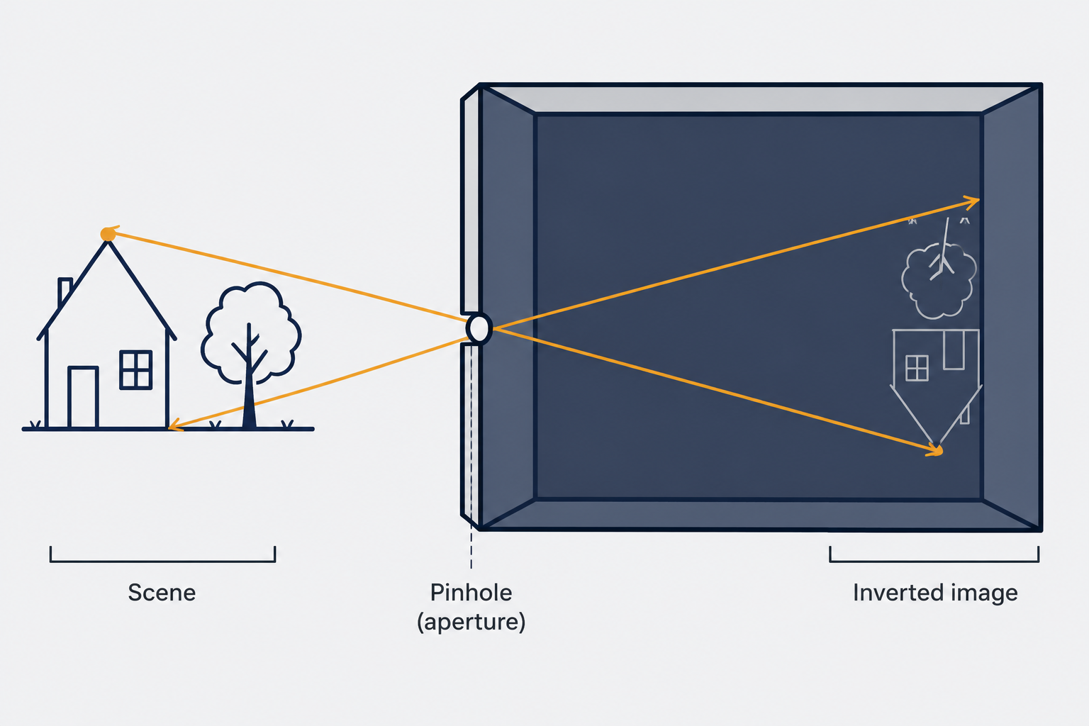
This is the essence of the pinhole camera model. A barrier with a small aperture sits between the 3D scene and the image surface (called the image plane or retinal plane). Only those rays that pass through the aperture reach the image plane. This enforces the crucial one-to-one correspondence between scene points and image points.

The Geometry and the Projection Equation

Let’s make this precise. We set up a coordinate system centered at the pinhole — which we call the optical center $O$. The three axes of this coordinate system, $\mathbf{i}$, $\mathbf{j}$, and $\mathbf{k}$, define what is known as the camera coordinate system. The axis $\mathbf{k}$ points perpendicularly toward the image plane, and the line connecting the optical center to the center of the image plane is called the optical axis.

The image plane sits at a distance $f$ from the pinhole — and this distance is one of the most important parameters in all of camera optics: the focal length.

Now consider a point $P = [x, y, z]^T$ in 3D space. Where does it land on the image plane? We can work this out using elementary geometry. The ray from $P$ through the pinhole $O$ hits the image plane at some point $P' = [x', y']^T$. Since the triangles formed by the ray on each side of the pinhole are similar, we can write:

\[P' = \begin{bmatrix} x' \\ y' \end{bmatrix} = \begin{bmatrix} f \frac{x}{z} \\ f \frac{y}{z} \end{bmatrix} \tag{1}\]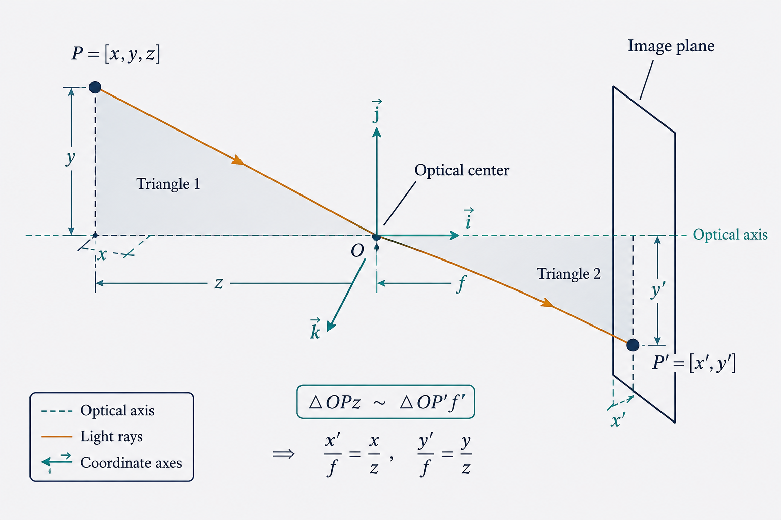

Here, $x$ and $y$ are the horizontal and vertical coordinates of the 3D point, $z$ is its depth (distance along the optical axis), and $f$ is the focal length. The fraction $\frac{x}{z}$ is exactly what you’d expect intuitively: a point that is twice as far away ($z$ doubles) appears to be half as far from the center of the image ($x'$ halves). This is the mathematical expression of perspective — the reason train tracks appear to converge in the distance.

Notice the critical nonlinearity: we are dividing by $z$. This means the mapping from 3D to 2D is not a simple linear transformation — a fact that will have important consequences for how we represent it in matrix form later.

The Aperture Dilemma

The pinhole model assumes the aperture is a mathematical point — infinitely small. In practice, this is impossible to achieve, and there is a fundamental tradeoff hiding here.

If the aperture is very small, the one-to-one mapping is nearly perfect and the image is sharp. But very little light gets through, making the image very dark. If the aperture is enlarged, more light enters, but now each point on the image plane receives rays from multiple scene points — the image blurs. This is the classic tension every photographer knows: aperture size controls both brightness and sharpness, and you cannot have both simultaneously without an additional optical element.

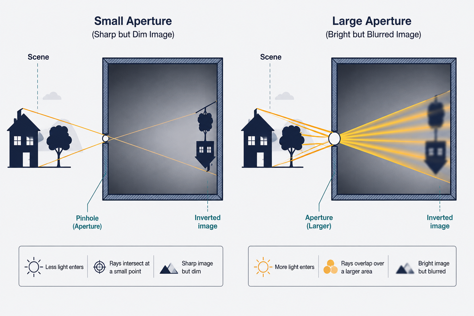
This tradeoff is what motivated the invention of lenses.

Lenses: Solving the Brightness-Sharpness Dilemma

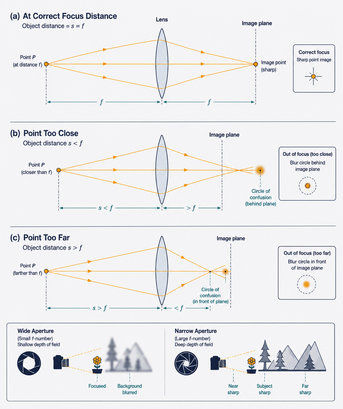
A lens is a piece of shaped glass that refracts (bends) light rays. A convex lens, properly designed and positioned, has a remarkable property: all the light rays emitted by a single scene point $P$, no matter what direction they travel when they hit the lens, are bent so that they all converge to the same image point $P’$ on the image plane.

This is the key insight. Without a lens, only the one ray that happened to be aimed at the tiny pinhole would contribute to forming the image. With a lens, the enormous number of rays radiating from $P$ across the full aperture of the lens all cooperate to illuminate the same image point $P’$. The image becomes dramatically brighter, without sacrificing the clean one-to-one mapping.

Lenses also have a special relationship with parallel rays: all light rays traveling parallel to the optical axis are focused by the lens to converge at a single point called the focal point. The distance from the lens center to the focal point is, again, the focal length $f$.

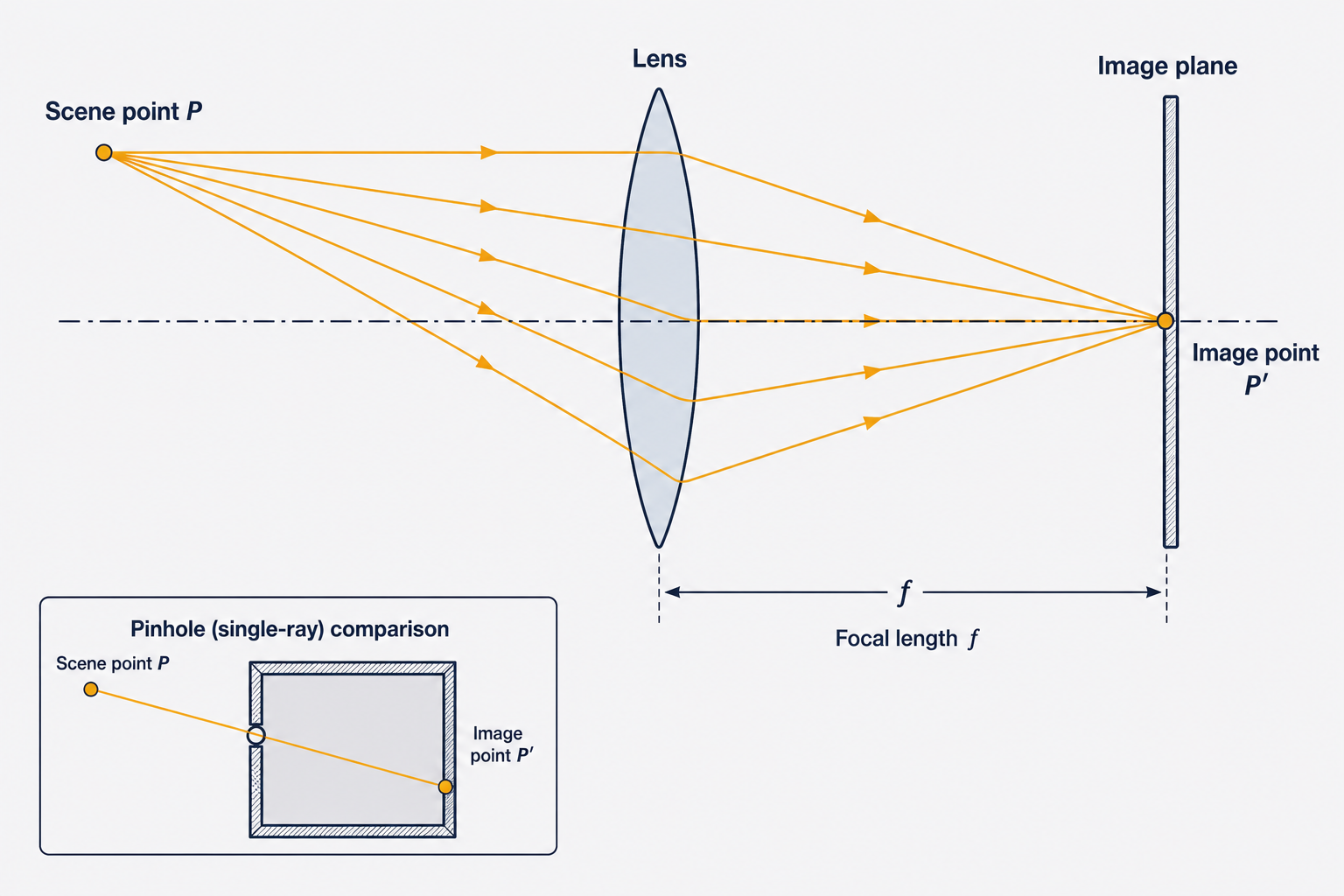
Using a simple geometric model of lens behavior (known as the paraxial refraction model, or thin lens approximation), one can derive a projection equation similar to the pinhole case:

\[P' = \begin{bmatrix} x' \\ y' \end{bmatrix} = \begin{bmatrix} \frac{z' x}{z} \\ \frac{z' y}{z} \end{bmatrix} \tag{2}\]

The key difference from the pinhole model is that instead of $z’ = f$, we now have $z’ = f + z_0$, where $z_0$ is the distance from the lens to the image plane. This extra term accounts for the fact that the lens refracts rather than simply blocks light.

Depth of Field and Focus

There is one important limitation with lenses: the perfect convergence to a single image point only works for scene points at a specific distance from the lens. Points that are closer or farther will not converge perfectly on the image plane — their rays will hit the plane while still spreading out, creating a blurred disk (called a circle of confusion). The range of distances over which objects appear acceptably sharp is called the depth of field.

This is why portrait photographers use wide apertures (for beautiful background blur) and landscape photographers use narrow apertures (to keep everything sharp from foreground to horizon). The mathematics of depth of field flows directly from the lens model we’ve just described.

Radial Distortion: When Lenses Aren’t Perfect

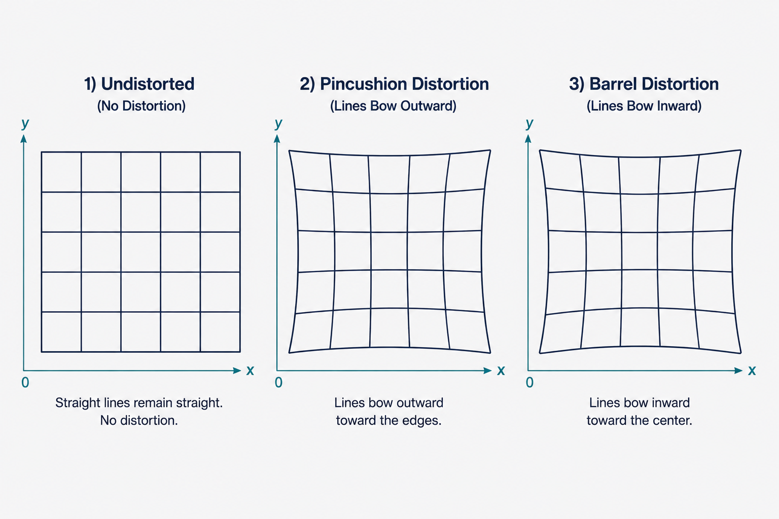
The paraxial (thin lens) approximation assumes that incoming rays make very small angles with the optical axis, allowing us to substitute $\sin(\theta) \approx \theta$. For wide-angle lenses or rays far from the center, this approximation breaks down, and real lenses introduce radial distortion.

Radial distortion causes the image magnification to vary as a function of distance from the optical center. When magnification increases away from the center, straight lines bow outward — this is called pincushion distortion. When magnification decreases away from the center, lines bow inward — this is called barrel distortion, the characteristic wide “fisheye” look. Both arise because different regions of the lens have slightly different effective focal lengths. This is a real-world imperfection that must be accounted for in precise computer vision applications.

From Image Plane to Digital Pixels: The Full Camera Model

The projection equation we derived maps a 3D point to a continuous 2D coordinate on the image plane. But a real digital image is not a continuous plane — it is a discrete grid of pixels, often with a different coordinate origin and possibly different physical units. Bridging this gap requires several additional steps.

Step 1: The Principal Point Offset

The image coordinate system in a pinhole camera has its origin at the principal point $C’$ — the point where the optical axis pierces the image plane, right at the center of the image. But digital images typically place their origin at the top-left or bottom-left corner. The displacement between these two origins is described by two parameters, $c_x$ and $c_y$ (in physical units), and the projection equation becomes:

\[P' = \begin{bmatrix} x' \\ y' \end{bmatrix} = \begin{bmatrix} f \frac{x}{z} + c_x \\ f \frac{y}{z} + c_y \end{bmatrix} \tag{3}\]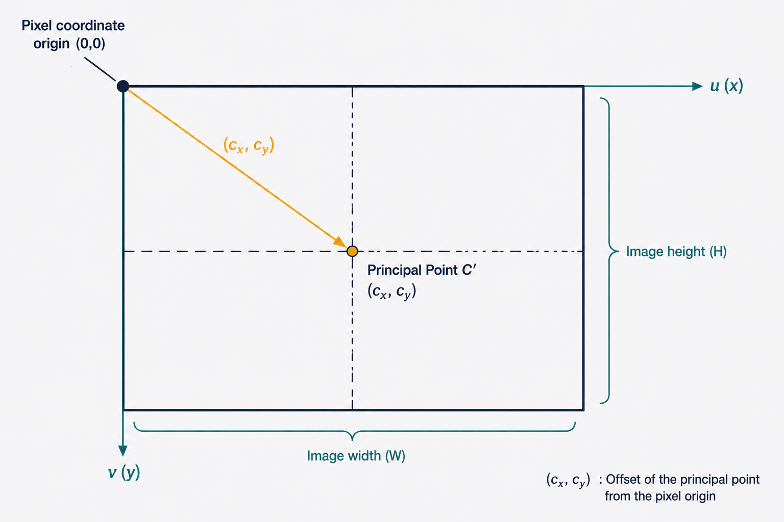

Step 2: Converting to Pixels

Points in the image plane are measured in physical units (millimeters, say), but pixels are discrete, dimensionless units. To convert, we introduce two scaling factors: $k$ and $l$, measured in pixels per unit length. These may differ from each other because pixels are not guaranteed to be perfectly square — the aspect ratio depends on the sensor. When $k = l$, we say the camera has square pixels.

We often fold $f$ and the scaling factors together into combined parameters $\alpha = fk$ and $\beta = fl$, giving:

\[P' = \begin{bmatrix} x' \\ y' \end{bmatrix} = \begin{bmatrix} \alpha \frac{x}{z} + c_x \\ \beta \frac{y}{z} + c_y \end{bmatrix} \tag{4}\]

Here $\alpha$ and $\beta$ are the focal lengths in units of pixels, which is how you will most commonly see them in practice.

Homogeneous Coordinates: Making Division into Multiplication

We now face a mathematical nuisance. The projection $P \to P’$ involves division by $z$, which means it cannot be written as a simple matrix-vector multiplication. Linear algebra is most powerful when we can write everything as $\mathbf{y} = M\mathbf{x}$, but our transformation stubbornly refuses to cooperate — or so it seems.

The elegant solution is a change of representation called homogeneous coordinates.

The idea is beautifully simple: append an extra coordinate. A 2D point $(x, y)$ becomes $(x, y, 1)$ in homogeneous coordinates. More generally, any point $(x, y, w)$ in homogeneous coordinates represents the Euclidean point $(x/w, y/w)$. Going back to Euclidean coordinates simply means dividing through by the last coordinate. And a 3D point $(x, y, z)$ becomes $(x, y, z, 1)$.

This trick allows us to absorb the problematic division into the coordinate system itself. Now we can write the full projection as a matrix-vector product:

\[P'_h = \begin{bmatrix} \alpha x + c_x z \\ \beta y + c_y z \\ z \end{bmatrix} = \begin{bmatrix} \alpha & 0 & c_x & 0 \\ 0 & \beta & c_y & 0 \\ 0 & 0 & 1 & 0 \end{bmatrix} \begin{bmatrix} x \\ y \\ z \\ 1 \end{bmatrix} \tag{5}\]

To recover the actual 2D pixel coordinates, we divide the first two entries by the third: $x’ = (\alpha x + c_x z)/z = \alpha x/z + c_x$, exactly as before. The division happens, but it is now hidden inside the conversion from homogeneous back to Euclidean coordinates.

From here on, all coordinates are assumed to be homogeneous unless stated otherwise.

The Camera Matrix $K$: Packaging the Intrinsic Parameters

We can factor the projection matrix cleanly:

\[P' = \begin{bmatrix} \alpha & 0 & c_x & 0 \\ 0 & \beta & c_y & 0 \\ 0 & 0 & 1 & 0 \end{bmatrix} P = \begin{bmatrix} \alpha & 0 & c_x \\ 0 & \beta & c_y \\ 0 & 0 & 1 \end{bmatrix} \begin{bmatrix} I & \mathbf{0} \end{bmatrix} P = K \begin{bmatrix} I & \mathbf{0} \end{bmatrix} P \tag{6}\]

The $3 \times 3$ matrix $K$ is called the camera matrix (or camera intrinsic matrix):

\[K = \begin{bmatrix} \alpha & -\alpha \cot\theta & c_x \\ 0 & \frac{\beta}{\sin\theta} & c_y \\ 0 & 0 & 1 \end{bmatrix} \tag{7}\]

The angle $\theta$ here accounts for skew — the possibility that the pixel axes are not perfectly perpendicular to each other, typically due to manufacturing imperfections. For most cameras, $\theta = 90°$, so $\cot\theta = 0$ and $\sin\theta = 1$, and the skew term vanishes.

In the general case with skew included, $K$ has exactly 5 degrees of freedom:

$\alpha$ and $\beta$: focal lengths in pixel units (2 parameters)
$c_x$ and $c_y$: principal point offset (2 parameters)
$\theta$ (or equivalently the skew value): pixel axis angle (1 parameter)

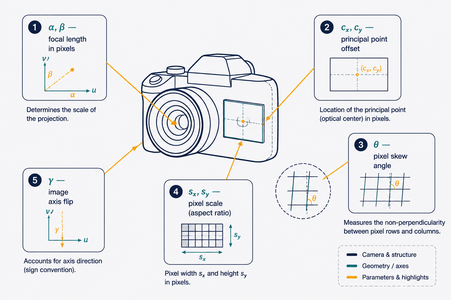
These five numbers, collectively called the intrinsic parameters, fully characterize the internal optics of a specific camera. They are properties of the camera itself — they change if you swap the lens or use a different sensor, but not if you point the camera in a different direction.

Extrinsic Parameters: Where Is the Camera in the World?

So far, we have described how a 3D point expressed in camera coordinates gets projected onto the image plane. But the 3D world has its own coordinate system — a world reference frame — that may be completely different from the camera’s local frame.

Think of it this way: a surveyed map of a city defines a world coordinate system. A camera placed somewhere in the city has its own local coordinate system. To project a building’s corner (specified in world coordinates) onto the camera’s image, we first need to convert that building corner from world coordinates to camera coordinates.

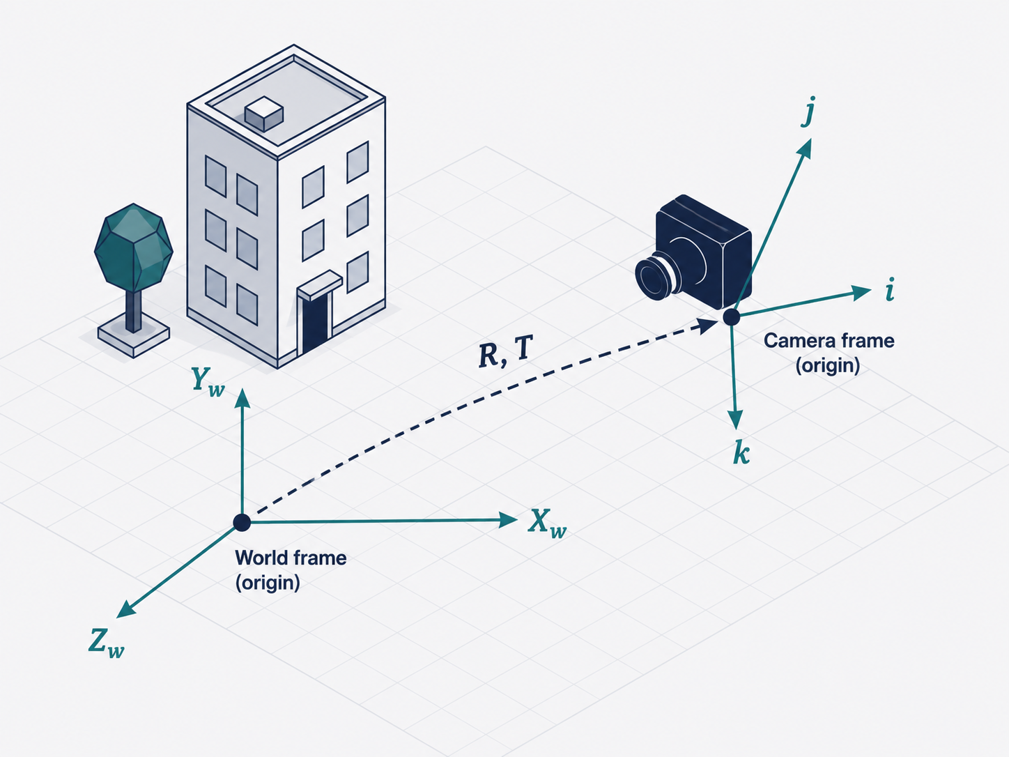
This coordinate transformation is captured by a rotation matrix $R$ (a $3 \times 3$ orthogonal matrix with determinant 1) and a translation vector $T$ (a 3D vector). Together they describe the camera’s position and orientation in the world. Given a point $P_w$ in world coordinates, its camera-frame coordinates are:

\[P = \begin{bmatrix} R & T \\ \mathbf{0} & 1 \end{bmatrix} P_w \tag{8}\]

Substituting this into our projection equation gives the complete pipeline from world point to pixel:

\[P' = K \begin{bmatrix} R & T \end{bmatrix} P_w = M P_w \tag{9}\]

The $3 \times 4$ matrix $M = K[R \mid T]$ is called the full projection matrix. It encodes everything about the camera — intrinsic and extrinsic.

$R$ and $T$ are the extrinsic parameters — they describe the camera’s pose in the world, not any intrinsic optical property. They change whenever you move or rotate the camera.

Counting degrees of freedom for the complete projection matrix: 5 from the intrinsic camera matrix $K$, 3 from the rotation $R$ (which can be parameterized by three Euler angles or equivalent), and 3 from the translation $T$ — giving 11 degrees of freedom in total. Remarkably, the entire geometry of a camera in the world can be described by just 11 numbers.

Camera Calibration: Recovering the Camera Parameters from Images

Knowing the projection matrix $M$ precisely is essential for many applications. In robotics, you need to know exactly where a detected object is in 3D space. In augmented reality, you need to overlay virtual objects on the real scene with perfect alignment. In photogrammetry, you reconstruct 3D structure from photographs. All of these require knowing $K$, $R$, and $T$.

The problem of estimating these parameters from images is called camera calibration.

The Setup: A Calibration Rig

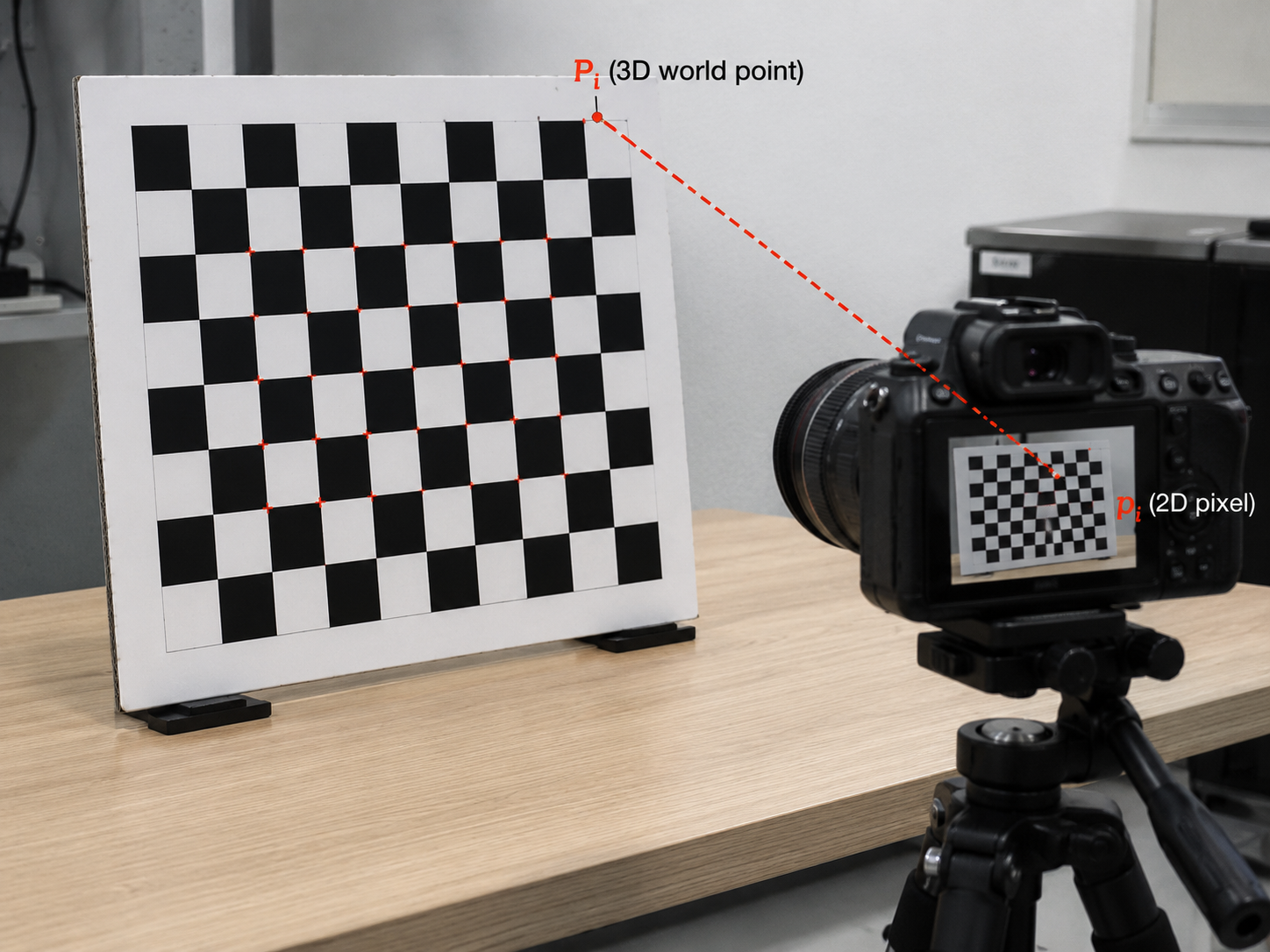
The standard approach uses a calibration rig — an object with a known, precisely measured 3D structure. The classic choice is a checkerboard pattern. Because we know the exact geometry of the checkerboard, we know the 3D world coordinates $P_1, P_2, \ldots, P_n$ of the grid corners. We then photograph the checkerboard and find the corresponding 2D pixel locations $p_1, p_2, \ldots, p_n$ in the image. Each pair $(P_i, p_i)$ is a correspondence.

Setting Up the Linear System

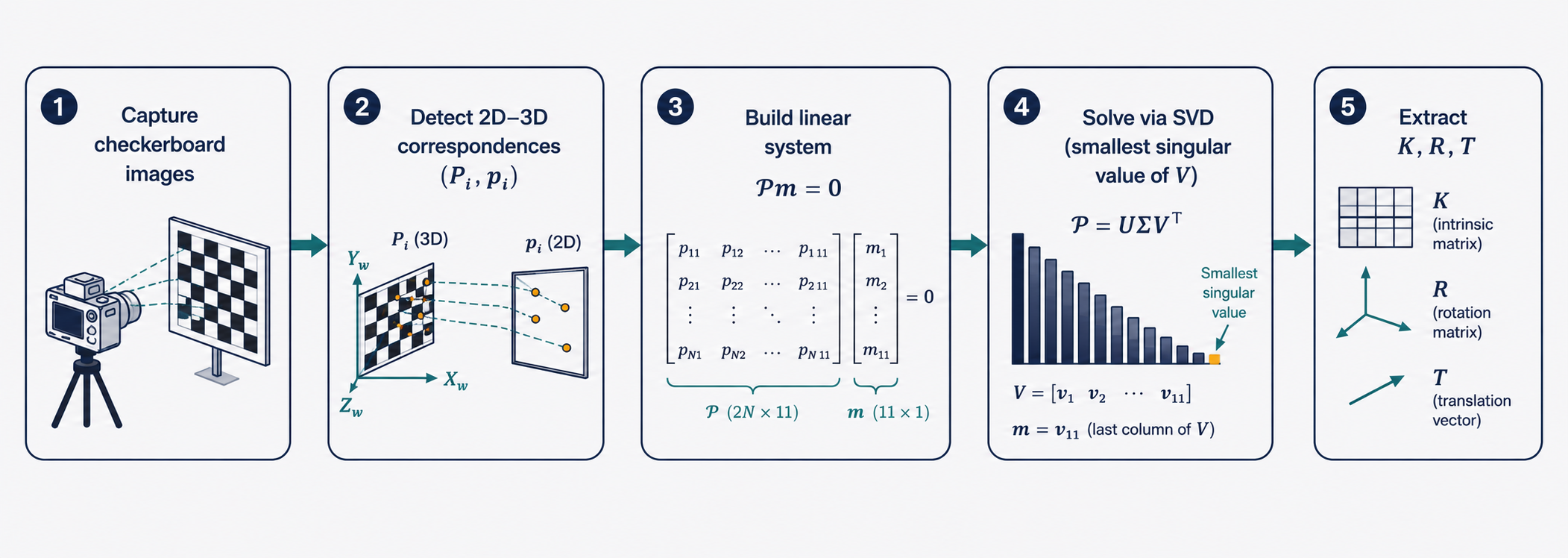
Each correspondence provides two equations. Given the projection $p_i = [u_i, v_i]^T = MP_i$, where $M$ has rows $\mathbf{m}_1^T, \mathbf{m}_2^T, \mathbf{m}_3^T$, we can write:

\[u_i = \frac{\mathbf{m}_1^T P_i}{\mathbf{m}_3^T P_i}, \qquad v_i = \frac{\mathbf{m}_2^T P_i}{\mathbf{m}_3^T P_i}\]

Rearranging to eliminate the denominator:

$u_i (\mathbf{m}_3^T P_i) - \mathbf{m}_1^T P_i = 0$ $v_i (\mathbf{m}_3^T P_i) - \mathbf{m}_2^T P_i = 0$

Stacking these equations for all $n$ correspondences gives a homogeneous linear system:

\[\mathcal{P}\mathbf{m} = \mathbf{0} \tag{10}\]

where $\mathbf{m}$ is a vector containing all 12 entries of $M$, and $\mathcal{P}$ is a $2n \times 12$ matrix built from the correspondence data.

Since $M$ has 11 degrees of freedom (and is only determined up to an overall scale), we need at least 6 correspondences to have more equations than unknowns ($2 \times 6 = 12 > 11$). In practice, many more are used to handle measurement noise.

Solving via SVD

The system $\mathcal{P}\mathbf{m} = \mathbf{0}$ has a trivial solution ($\mathbf{m} = \mathbf{0}$), which is useless. We add the constraint $|\mathbf{m}|^2 = 1$ to prevent this, and solve the minimization:

\[\min_{\mathbf{m}} \|\mathcal{P}\mathbf{m}\|^2 \quad \text{subject to} \quad \|\mathbf{m}\|^2 = 1 \tag{11}\]

This is solved elegantly using Singular Value Decomposition (SVD). If $\mathcal{P} = UDV^T$, the solution is the last column of $V$ — the right singular vector corresponding to the smallest singular value. This vector is the direction in the null space of $\mathcal{P}$ that best approximates a zero, given noisy data.

Extracting Intrinsics and Extrinsics

After reshaping $\mathbf{m}$ back into the matrix $M$, we know $M$ up to a global scale factor $\rho$. From this scaled matrix, we can algebraically recover the individual intrinsic and extrinsic parameters:

\[\rho = \pm \frac{1}{\|\mathbf{a}_3\|}, \quad c_x = \rho^2 (\mathbf{a}_1 \cdot \mathbf{a}_3), \quad c_y = \rho^2 (\mathbf{a}_2 \cdot \mathbf{a}_3)\] \[\theta = \cos^{-1}\!\left(- \frac{(\mathbf{a}_1 \times \mathbf{a}_3) \cdot (\mathbf{a}_2 \times \mathbf{a}_3)}{\|\mathbf{a}_1 \times \mathbf{a}_3\| \cdot \|\mathbf{a}_2 \times \mathbf{a}_3\|}\right)\] \[\alpha = \rho^2 \|\mathbf{a}_1 \times \mathbf{a}_3\| \sin\theta, \quad \beta = \rho^2 \|\mathbf{a}_2 \times \mathbf{a}_3\| \sin\theta \tag{12}\]

The extrinsic parameters follow from:

\[\mathbf{r}_3 = \rho \mathbf{a}_3, \quad \mathbf{r}_1 = \frac{\mathbf{a}_2 \times \mathbf{a}_3}{\|\mathbf{a}_2 \times \mathbf{a}_3\|}, \quad \mathbf{r}_2 = \mathbf{r}_3 \times \mathbf{r}_1, \quad T = \rho K^{-1} \mathbf{b} \tag{13}\]

where $\mathbf{a}_1^T, \mathbf{a}_2^T, \mathbf{a}_3^T$ are the rows of the $3 \times 3$ left submatrix of $M$, and $\mathbf{b}$ is its last column.

Degenerate Configurations

Not every set of correspondences will work. If all the calibration points happen to lie on a single plane, the system becomes degenerate and cannot be solved — there are infinitely many projection matrices consistent with planar point sets. More generally, degenerate configurations arise whenever points lie on the intersection curve of two quadric surfaces. This is why checkerboard calibration rigs are designed to be three-dimensional, often captured from multiple angles, ensuring the points span 3D space.

Handling Distortion in Calibration

Real lenses deviate from the ideal pinhole model. The most common imperfection is radial distortion, which warps the image in a way that is symmetric around the optical center.

We can model this distortion with an isotropic scaling factor $\lambda$ that depends on the distance from the image center:

\[Q P_i = \begin{bmatrix} \frac{1}{\lambda} & 0 & 0 \\ 0 & \frac{1}{\lambda} & 0 \\ 0 & 0 & 1 \end{bmatrix} M P_i = p_i \tag{14}\]

Unfortunately, introducing this distortion model makes the calibration system nonlinear — $\lambda$ itself may be a function of image position, so we can no longer use SVD directly. However, there is a useful observation: radial distortion does not affect the ratio $u_i / v_i$, since both coordinates are divided by the same $\lambda$. This allows us to estimate the first two rows of $M$ using a linear system (solvable by SVD), and then recover the third row and $\lambda$ through a simpler nonlinear optimization. The full nonlinear distortion problem is thus reduced to a more tractable form.

Alternative Camera Models: When Perspective Is Overkill

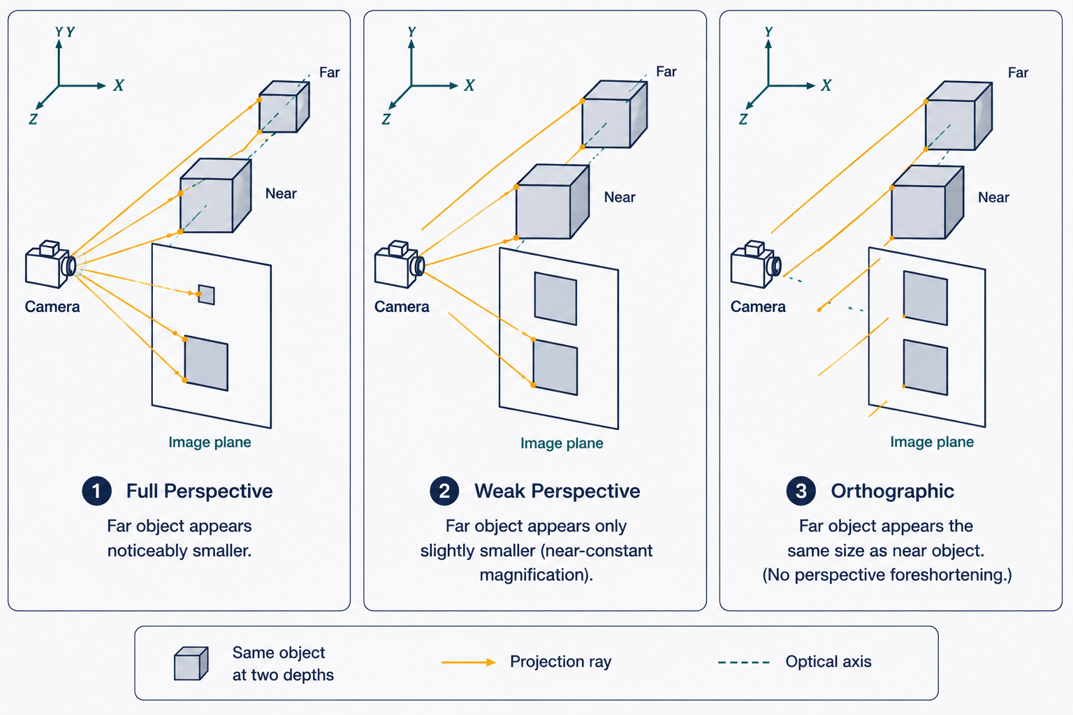
The perspective (pinhole) camera model is accurate, but computationally rich. In some scenarios, simpler approximations are sufficient and much more convenient to work with.

The Weak Perspective Model

Imagine you are photographing an object that is relatively small compared to its distance from the camera. In this case, the variation in depth across the object — from its nearest point to its farthest — is tiny compared to the overall distance $z_0$. Under these conditions, the perspective division by $z$ can be replaced by division by the fixed reference depth $z_0$, giving a constant magnification across the entire object:

\[x' = \frac{f'}{z_0} x, \qquad y' = \frac{f'}{z_0} y\]

The ratio $m = f’/z_0$ is just a single magnification constant. This is the weak perspective model. It simplifies the projection matrix so that the bottom row becomes $[0\ 0\ 0\ 1]$ rather than the variable expression in the full perspective model. The beautiful consequence is that the nonlinearity of projection disappears entirely — the transformation becomes a simple linear magnification, independent of depth.

The projection in the weak perspective model takes the clean form:

\[P' = MP = \begin{bmatrix} m_1 \\ m_2 \\ m_3 \end{bmatrix} P = \begin{bmatrix} m_1 P \\ m_2 P \\ 1 \end{bmatrix} \tag{15}\]

Each image coordinate is just a linear function of the 3D point coordinates. No division, no depth dependence. This makes many algorithms dramatically simpler while remaining accurate for small, distant objects.

The Orthographic Projection Model

Pushing the approximation even further, if the camera is conceptually placed at infinity (the optical center recedes infinitely far from the scene), all projection rays become parallel and perpendicular to the image plane. The image coordinates are simply the $x$ and $y$ coordinates of the 3D point, with no scaling whatsoever:

\[x' = x, \qquad y' = y\]

This is the orthographic projection model (also called affine projection). Depth is completely ignored — an object 10 meters away looks exactly the same as one 100 meters away, as long as their $x$ and $y$ coordinates match. This is clearly unrealistic for most photography, but it is the standard model in architectural drawings and engineering schematics, where preserving true proportions without perspective distortion is the goal.

Think of a blueprint: a room drawn in orthographic projection allows you to directly measure distances on paper and map them to real-world distances with a single scale factor. No correction for perspective is needed.

Rigid Transformations: The Mathematics of Moving Through Space

Underpinning the entire discussion is a family of geometric operations called rigid transformations — transformations that preserve distances and angles. The key ones are rotation, translation, and scaling.

Rotation

A rotation in 3D can be described as a combination of rotations around the three coordinate axes. The rotation matrices for each axis are:

\[R_x(\alpha) = \begin{bmatrix} 1 & 0 & 0 \\ 0 & \cos\alpha & -\sin\alpha \\ 0 & \sin\alpha & \cos\alpha \end{bmatrix}, \quad R_y(\beta) = \begin{bmatrix} \cos\beta & 0 & \sin\beta \\ 0 & 1 & 0 \\ -\sin\beta & 0 & \cos\beta \end{bmatrix}\] \[R_z(\gamma) = \begin{bmatrix} \cos\gamma & -\sin\gamma & 0 \\ \sin\gamma & \cos\gamma & 0 \\ 0 & 0 & 1 \end{bmatrix}\]

These are called Euler angle rotations. To rotate first around $z$, then $y$, then $x$, you apply the matrix product $R_x R_y R_z$. Note that rotation matrices are orthogonal ($R^T R = I$) with determinant 1 — they perfectly preserve lengths and angles.

One important subtlety: Euler angles can lead to a problem called gimbal lock, where certain configurations cause a loss of a rotational degree of freedom (two of the three axes become aligned, reducing 3D rotation to a 2D one). This is why many robotics and aerospace systems use alternative representations like quaternions.

Translation and Combined Transformations

Translation simply shifts a point by a vector $\mathbf{t} = [t_x, t_y, t_z]^T$:

\[P' = P + \mathbf{t}\]

In homogeneous coordinates, this can be written as a matrix multiplication using the translation matrix:

\[T = \begin{bmatrix} 1 & 0 & 0 & t_x \\ 0 & 1 & 0 & t_y \\ 0 & 0 & 1 & t_z \\ 0 & 0 & 0 & 1 \end{bmatrix}\]

The power of homogeneous coordinates is that we can now chain rotations, translations, and scalings together by simply multiplying matrices — every transformation in the pipeline becomes a matrix, and the full pipeline is their product. The final combined transformation matrix for rotating by $R$, scaling by $S$, and translating by $\mathbf{t}$ is:

\[T_{\text{combined}} = \begin{bmatrix} RS & \mathbf{t} \\ \mathbf{0} & 1 \end{bmatrix}\]

All of these rotation, translation, and scaling operations are examples of affine transformations (they preserve parallel lines). The full perspective projection, however, is a projective transformation, distinguished by the fact that the bottom row of the matrix is not simply $[0\ 0\ 0\ 1]$ — this is precisely the term responsible for the perspective division by $z$.

Putting It All Together: The Complete Projection Pipeline

Let’s step back and appreciate the full picture. Starting from a 3D point $P_w$ in the world:

Rigid transformation ($R$, $T$): Convert from world coordinates to camera coordinates. This accounts for where the camera is positioned and how it is oriented in the world.
Perspective projection: Project the 3D camera-frame point onto the 2D image plane using the focal length, encoding the geometry of the pinhole (or lens).
Intrinsic calibration ($K$): Apply the camera matrix to account for pixel scaling ($\alpha$, $\beta$), principal point offset ($c_x$, $c_y$), and potential skew ($\theta$). This converts from idealized image plane coordinates to actual pixel coordinates in the digital image.

The entire pipeline is:

\[P' = K \begin{bmatrix} R & T \end{bmatrix} P_w \tag{16}\]

This compact equation is arguably the most important formula in all of computer vision. Every photograph ever taken by a digital camera is, in some sense, an instance of this equation being applied to a 3D scene.

Why This All Matters: Practical Implications

Understanding camera models is not academic abstraction — it has immediate, concrete consequences for any system that works with images.

In autonomous vehicles, the cameras mounted on the car must have precisely known intrinsic and extrinsic parameters so that detected objects (pedestrians, traffic lights, road markings) can be accurately localized in 3D space relative to the vehicle. A calibration error of even a few pixels can translate to errors of tens of centimeters in 3D position estimates — potentially catastrophic at highway speeds.

In augmented reality, virtual objects must be rendered with the same perspective, focal length, and distortion as the real camera. If the intrinsic parameters are slightly off, virtual objects will seem to “float” or “slide” relative to the real world as you move your head. The illusion depends entirely on precise calibration.

In 3D reconstruction (photogrammetry, structure-from-motion), multiple photographs taken from different angles are used to reconstruct the 3D geometry of a scene. This is only possible because each photograph encodes the projection geometry through the camera model, and those projections can be inverted — with sufficient correspondences — to recover the 3D structure.

In medical imaging, calibration matters when cameras are used in surgical robotics or endoscopy, where the precise mapping between image coordinates and physical space can mean the difference between a successful procedure and a dangerous mistake.

Conclusion: A Mathematical Window on the World

We began with a simple observation — a pinhole in a barrier creates an image — and ended with a complete mathematical framework for understanding how any camera maps the 3D world to a 2D image. Along the way, we discovered that:

The pinhole model gives us the fundamental perspective projection $x’ = fx/z$, capturing the essence of how depth creates apparent size. Lenses resolve the practical tension between brightness and sharpness, while introducing distortions that must be modeled and corrected. The camera matrix $K$ packages the five intrinsic parameters that characterize a camera’s optics, while the rotation $R$ and translation $T$ describe its pose in the world. Homogeneous coordinates provide the algebraic sleight-of-hand that lets us write the nonlinear perspective projection as a linear matrix multiplication. Camera calibration recovers all these parameters from images of known calibration targets, using the elegant machinery of SVD. And simplified models like weak perspective and orthographic projection offer useful approximations when the full perspective model is more than we need.

Every time you take a photo, run a face detection algorithm, or watch an autonomous car navigate traffic, this mathematics is silently at work — encoding the geometry of light, space, and optics into the numbers that machines can reason about. Understanding camera models is, in a real sense, understanding how computers learn to see.

This article is based on CS231A Course Notes 1: Camera Models, by Kenji Hata and Silvio Savarese, Stanford University.

Camera Models