Two Eyes Are Better Than One: A Deep Dive into Epipolar Geometry

Two Eyes Are Better Than One: A Deep Dive into Epipolar Geometry

How the geometric relationship between two cameras lets us reconstruct 3D scenes, match points across images, and “straighten” any stereo pair — without ever measuring the physical world.

There is a simple experiment you can perform right now. Hold your finger up in front of your face, close one eye, and align your finger with some object in the background — say, a door frame. Now switch eyes. Your finger appears to have jumped to a different position relative to the door frame. The door frame itself, being far away, barely moves. Your nearby finger shifts dramatically.

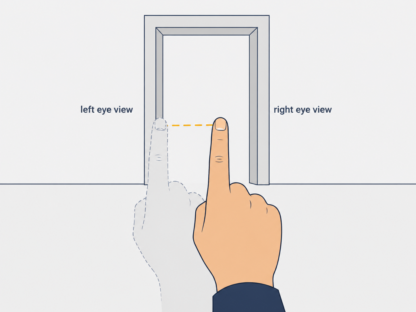
This everyday phenomenon — called parallax — is the fundamental intuition behind stereoscopic vision. The difference in an object’s apparent position between two viewpoints encodes, with mathematical precision, how far away that object is. Two eyes, two cameras, or one camera moved between two shots can all exploit this principle. But to do so rigorously, we need a mathematical framework that describes exactly how the geometry of two viewpoints constrains what we can see and where.

That framework is epipolar geometry. It is one of the foundational pillars of computer vision and 3D reconstruction, and its elegance lies in this: without knowing where a 3D point is, and without even knowing the properties of the cameras involved, epipolar geometry tells us that if a point appears at a specific pixel in one image, it can only appear somewhere along a specific line in the other image. This “epipolar constraint” turns an overwhelming 2D search problem into a 1D one, and it unlocks a chain of algorithms for matching images, estimating camera geometry, and ultimately reconstructing the 3D world.

The Limits of a Single View

Before diving into the geometry of two cameras, it is worth understanding precisely why one image isn’t enough. When a camera projects the 3D world onto a flat image sensor, it performs a projection along rays. Every point along a ray from the camera center through a pixel maps to the same pixel. Depth — the distance along that ray — is simply lost. This is the intrinsic ambiguity of perspective projection.

This ambiguity creates visual illusions that are trivially resolved by a second viewpoint. A famous class of such illusions involves forced perspective photography: a person appears to be holding up the Leaning Tower of Pisa because their hand and the tower, at vastly different depths, happen to project onto the same image region. Viewed from a second camera at a different angle, the deception collapses immediately. The spatial relationship between the person and the tower is unambiguous from two views.

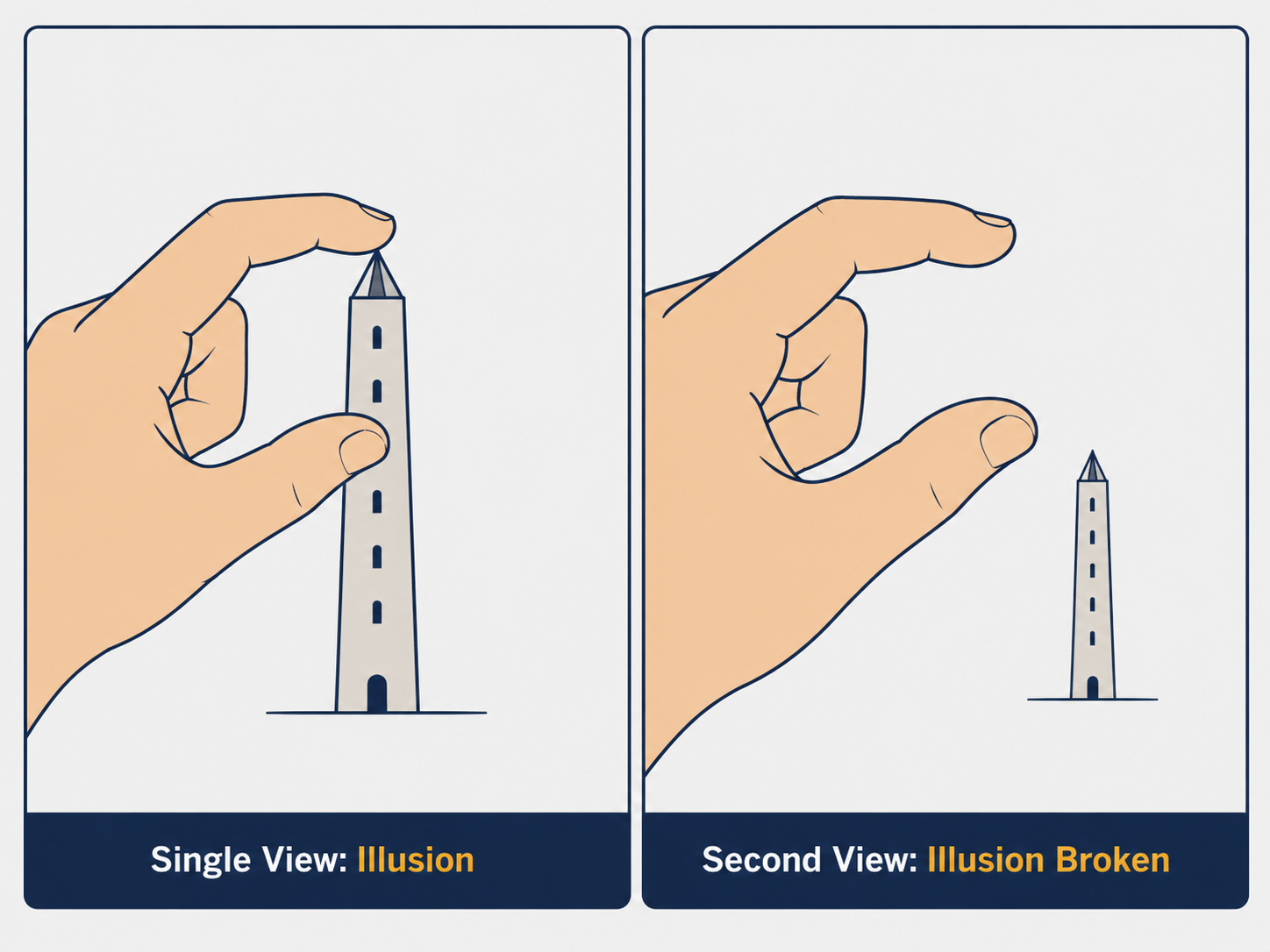
The mathematical goal, then, is to formalize what a pair of images tells us that a single image cannot.

Part 1: The Epipolar Geometry Setup

The Five Key Elements

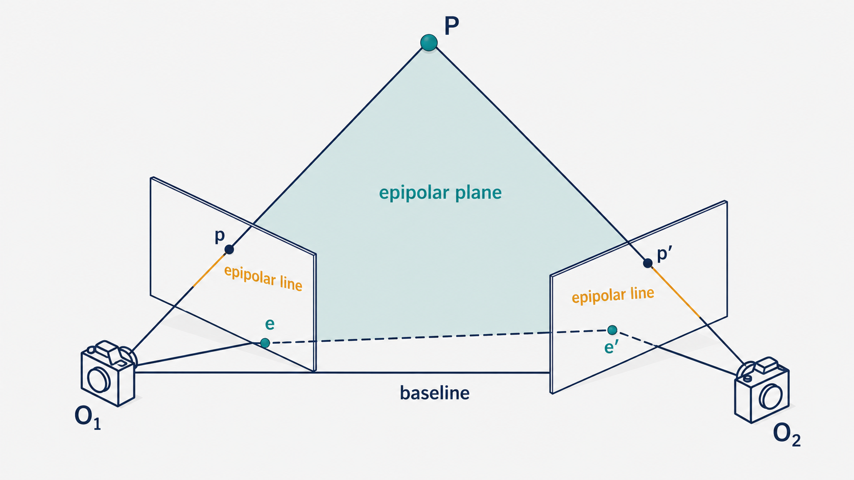
Imagine two cameras — call their optical centers $O_1$ and $O_2$ — both observing the same 3D point $P$. The point $P$ projects to pixel $p$ in the first image and pixel $p’$ in the second image. This simple scenario generates a beautifully structured geometry involving five elements:

The baseline is the line segment connecting the two camera centers $O_1$ and $O_2$. Think of it as the physical separation between the two cameras.

The epipolar plane is the triangle formed by the two camera centers and the 3D point $P$: the plane passing through $O_1$, $O_2$, and $P$. Every corresponding point pair $(p, p’)$ defines its own epipolar plane, but they all share the baseline.

The epipoles $e$ and $e’$ are where the baseline pierces each image plane. In physical terms, $e$ is where camera $O_2$ would appear if it were visible to camera $O_1$ (and vice versa). The epipoles are the projections of each camera center into the other camera’s image.

The epipolar lines are the intersections of the epipolar plane with each image plane. In each image, the epipolar line passes through the corresponding image point ($p$ or $p’$) and through the epipole. All epipolar lines in a given image fan out from the same epipole.

The Epipolar Constraint — Why It Matters

Here is the central insight. Suppose you are given the pixel location $p$ in the first image, and you want to find the corresponding pixel $p’$ in the second image (i.e., the pixel that depicts the same 3D point $P$). Without any geometric knowledge, you would have to search every pixel in the second image — an exhaustive 2D search. That’s computationally expensive, especially for high-resolution images.

Epipolar geometry reduces this search to a single line. Because $P$, $O_1$, and $O_2$ all lie in the epipolar plane, the projection of $P$ into the second camera ($p’$) must lie on the intersection of that epipolar plane with the second image plane — the epipolar line. Knowing $p$ in the first image (along with the camera geometry) uniquely determines the epipolar line in the second image. The search for $p’$ is reduced from a 2D area to a 1D line.

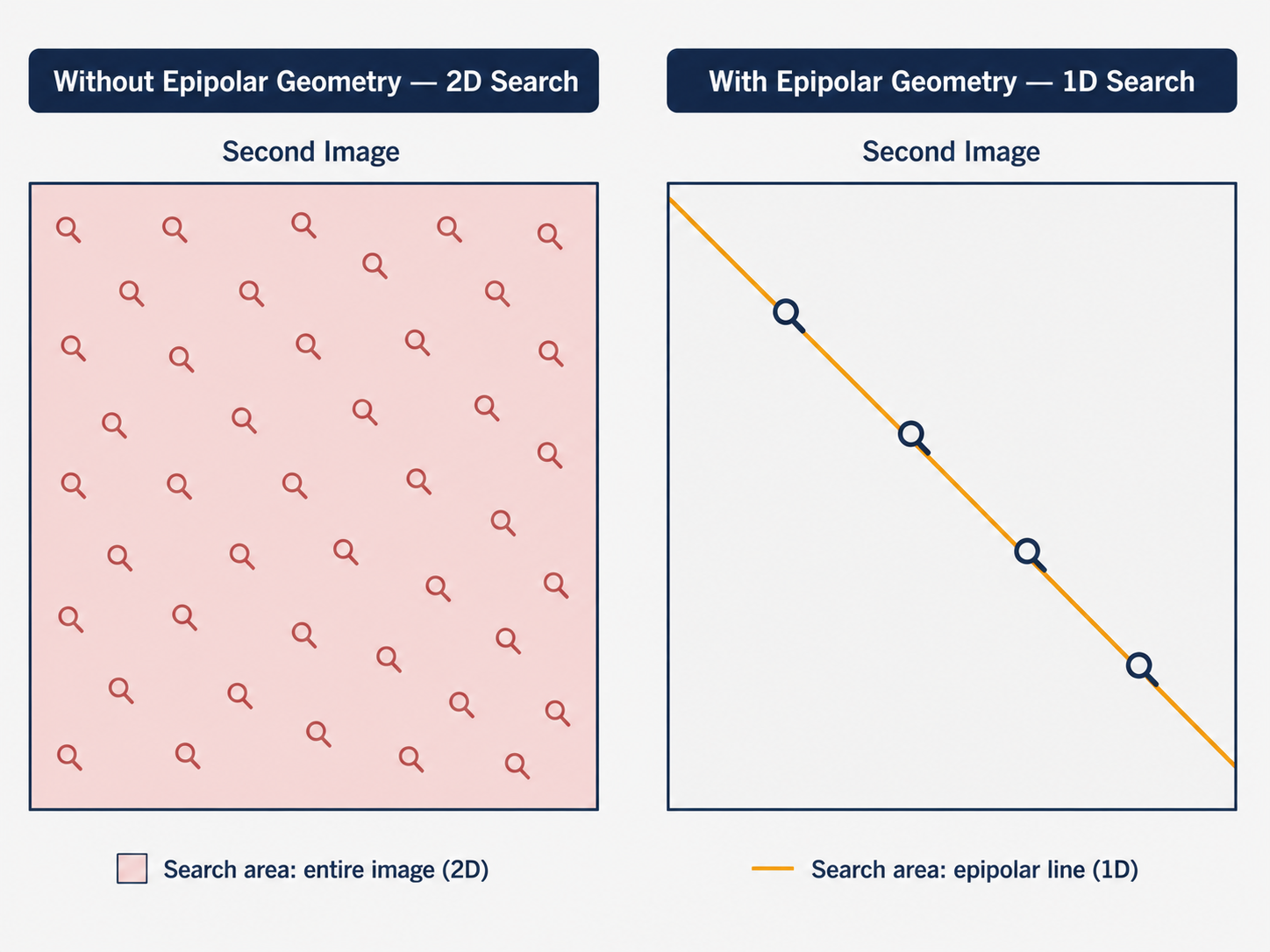
This matters enormously in practice. Stereo matching, 3D reconstruction, and structure-from-motion all rely fundamentally on the epipolar constraint to make correspondence search tractable.

A Special Case: Parallel Cameras

A particularly elegant special case arises when the two image planes are parallel to each other, with the baseline running horizontally between them. In this configuration, the baseline never intersects either image plane (it runs parallel to them), so the epipoles are pushed to infinity. The epipolar lines become perfectly horizontal — parallel to the $u$-axis of each image.

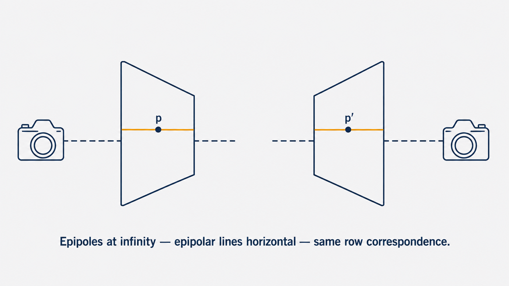
The consequence is beautifully simple: if a point appears at row $v$ in the first image, its corresponding point in the second image is guaranteed to appear at the same row $v$. The search is reduced from a 2D area to a single row. This is the ideal configuration for stereo cameras, and it is the target of a process called image rectification, which we’ll discuss at length later.

Part 2: The Essential Matrix — Encoding Geometry for Calibrated Cameras

Building the Constraint

Let’s now derive the mathematical form of the epipolar constraint. We begin with the simplest case: canonical cameras, where both cameras have identity intrinsic matrices ($K = K’ = I$). This means image coordinates are the same as coordinates in the camera’s reference frame — we’ve removed the complication of focal length, pixel size, and principal point for now.

We place the first camera at the origin, so its projection matrix is simply $M = [I \mid 0]$. The second camera is offset by a rotation $R$ and translation $T$, giving $M’ = [R^T \mid -R^T T]$.

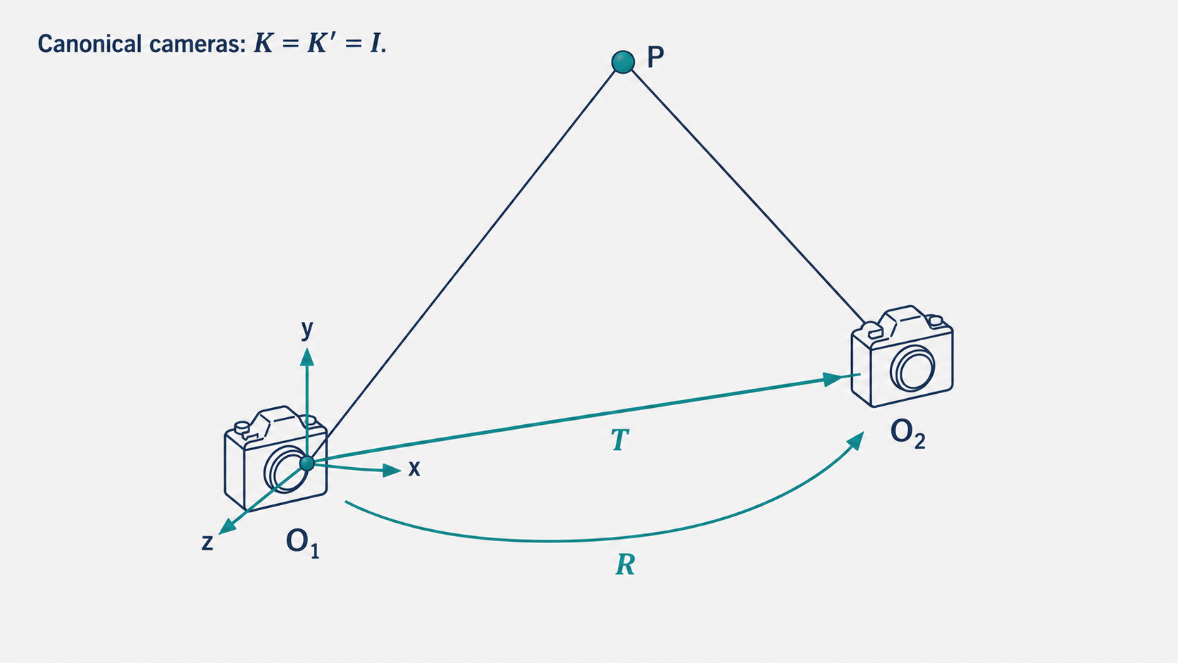
Now, consider the 3D point $P$ and its projections $p$ (in camera 1) and $p’$ (in camera 2). Since these are canonical cameras, $p$ and $p’$ are actual 3D ray directions, not pixel coordinates. The location of $p’$ expressed in camera 1’s reference frame is $Rp’ + T$.

Because $P$, $O_1$, and $O_2$ all lie in the epipolar plane, two vectors that lie in that plane are $T$ (from $O_1$ to $O_2$) and $Rp’ + T$ (from $O_1$ to $P$). Their cross product $T \times (Rp’ + T) = T \times Rp’$ is normal to the epipolar plane. Since $p$ also lies in the epipolar plane, it must be perpendicular to this normal:

\[p^T \cdot [T \times (Rp')] = 0\]

Introducing the Cross Product Matrix

To make this algebraically cleaner, we use a standard trick from linear algebra: the cross product of any vector $a$ with another vector $b$ can be written as a matrix-vector multiplication:

\[a \times b = \begin{bmatrix} 0 & -a_z & a_y \\ a_z & 0 & -a_x \\ -a_y & a_x & 0 \end{bmatrix} b = [a_\times] b\]

The matrix $[a_\times]$ is called the cross product matrix (or skew-symmetric matrix) of $a$. Using this notation, the epipolar constraint becomes:

\[p^T [T_\times] R p' = 0\]

The Essential Matrix

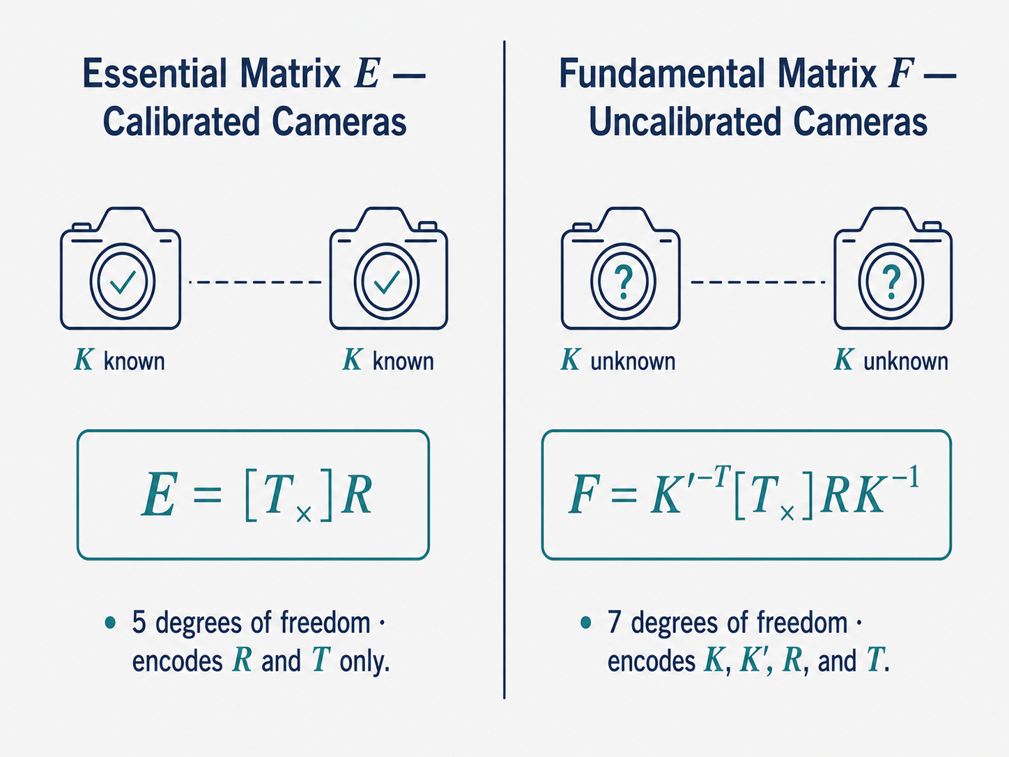
The matrix $E = [T_\times] R$ is called the Essential Matrix. The epipolar constraint takes the remarkably compact form:

\[p^T E p' = 0\]

This $3 \times 3$ matrix encodes everything about the relative geometry between the two cameras — the rotation $R$ and translation $T$ — in a single object. Let’s unpack what it can do.

Given the Essential matrix and a point $p$ in the first image, the epipolar line in the second image is $\ell’ = E^T p$. Conversely, given $p’$ in the second image, the epipolar line in the first image is $\ell = E p’$. You can verify this: if $p’$ lies on $\ell’$, then $p’^T \ell’ = p’^T E^T p = (p^T E p’)^T = 0$ ✓.

The Essential matrix also has a special relationship with the epipoles. Since every epipolar line in the second image passes through the epipole $e’$, and $e’$ lies on every epipolar line, we have $E e’ = 0$ and $E^T e = 0$. The epipoles are in the null space of $E$ and $E^T$ respectively.

Structurally, $E$ has 5 degrees of freedom (the rotation $R$ contributes 3, the translation direction $T/|T|$ contributes 2 — we can only recover the direction of translation, not its scale, from the images alone), it has rank 2 (one singular value is zero, corresponding to the null space direction of the epipole), and it is always singular.

Part 3: The Fundamental Matrix — Epipolar Geometry Without Calibration

Beyond Canonical Cameras

The Essential matrix is elegant, but it assumes we know the intrinsic calibration matrices $K$ and $K’$ of both cameras. In many real-world scenarios — photographs downloaded from the internet, images from unknown cameras, historical photos — we don’t have access to calibration information. Can we still reason about epipolar geometry?

Yes. The answer is the Fundamental Matrix, the generalization of the Essential matrix to uncalibrated cameras.

Recall that for non-canonical cameras, the projection matrices are $M = K[I \mid 0]$ and $M’ = K’[R^T \mid -R^T T]$. We can “undo” the calibration by defining $p_c = K^{-1} p$ and $p’_c = K’^{-1} p’$ — these are the image coordinates that would be observed if the cameras were canonical. The Essential matrix constraint then gives:

\[p_c^T [T_\times] R p'_c = 0\] \[\Rightarrow \quad p^T K^{-T} [T_\times] R K'^{-1} p' = 0\]

The matrix sandwiched between $p^T$ and $p’$ is the Fundamental Matrix:

\[F = K'^{-T} [T_\times] R K^{-1}\]

And the epipolar constraint in the uncalibrated case is:

\[p^T F p' = 0\]

What the Fundamental Matrix Encodes

The Fundamental matrix is a $3 \times 3$ matrix with 7 degrees of freedom. (It has 9 entries, determined only up to scale, reducing to 8; and the constraint $\det F = 0$ reduces it to 7.) It encodes not just the relative camera geometry ($R$, $T$) but also the intrinsic parameters of both cameras ($K$, $K’$).

Like the Essential matrix, $F$ maps points to epipolar lines: $\ell’ = F^T p$ gives the epipolar line in the second image, and $\ell = F p’$ gives the epipolar line in the first. The epipoles satisfy $F^T e = 0$ and $F e’ = 0$.

The most powerful aspect of $F$ is this: if we can estimate the Fundamental matrix directly from image correspondences (without knowing $K$, $R$, or $T$), then we gain the ability to compute epipolar lines for any pair of images, purely from observed pixel coordinates. This is what makes the Fundamental matrix the workhorse of uncalibrated stereo and structure-from-motion.

Part 4: The Eight-Point Algorithm — Estimating F from Correspondences

The Setup

The Eight-Point Algorithm (proposed by Longuet-Higgins in 1981, extended by Hartley in 1995) answers a practical question: given two photographs of the same scene, with no knowledge of the cameras, how can we estimate the Fundamental matrix?

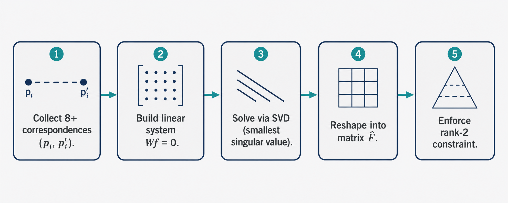
The input is a set of corresponding point pairs $(p_i, p’_i)$: pixel locations in both images that depict the same 3D point. Finding such correspondences is itself a challenge (handled by feature detection algorithms like SIFT or ORB), but assuming we have them, each correspondence gives us one equation from the epipolar constraint:

\[p_i^T F p'_i = 0\]

If we write $p_i = (u_i, v_i, 1)$ and $p’i = (u’_i, v’_i, 1)$ and expand $F$ into its 9 entries $F{jk}$, this constraint becomes a linear equation in the entries of $F$:

\[\begin{bmatrix} u_i u'_i & v'_i u_i & u_i & u'_i v_i & v_i v'_i & v_i & u'_i & v'_i & 1 \end{bmatrix} \begin{bmatrix} F_{11} \\ F_{12} \\ F_{13} \\ F_{21} \\ F_{22} \\ F_{23} \\ F_{31} \\ F_{32} \\ F_{33} \end{bmatrix} = 0\]

Each correspondence contributes one such row. Stacking $N$ correspondences gives the matrix equation:

\[W \mathbf{f} = 0\]

where $W$ is an $N \times 9$ matrix and $\mathbf{f}$ is the 9-vector of $F$’s entries. Since $F$ is determined only up to scale, we have 8 effective unknowns, requiring at least 8 correspondences — hence the name “Eight-Point Algorithm.”

Solving via SVD

With 8 or more correspondences, this is a homogeneous linear system. The solution is found via Singular Value Decomposition (SVD): we decompose $W = U \Sigma V^T$ and take the column of $V$ corresponding to the smallest singular value as the solution $\mathbf{f}$, then reshape it into the $3 \times 3$ matrix $\hat{F}$.

However, $\hat{F}$ may have rank 3 (full rank), whereas the true Fundamental matrix must have rank 2 (it must be singular, since the epipoles lie in its null space). We enforce this by finding the best rank-2 approximation: decompose $\hat{F} = U\Sigma V^T$, set the smallest singular value to zero, and recompose:

\[F = U \begin{bmatrix} \Sigma_1 & 0 & 0 \\ 0 & \Sigma_2 & 0 \\ 0 & 0 & 0 \end{bmatrix} V^T\]

This is the closest rank-2 matrix to $\hat{F}$ in the Frobenius norm sense — the mathematically optimal way to enforce the rank constraint.

Why the Naive Version Fails — and the Normalized Fix

The standard Eight-Point Algorithm as described has a significant practical problem: it produces poor results on real images. The culprit is numerical ill-conditioning.

Modern cameras have image coordinates in the range of thousands of pixels — for example, a 1920×1080 image has $u$ values up to 1920 and $v$ values up to 1080. When these large numbers are multiplied together to form the entries of $W$ (products like $u_i u’_i$ reach values in the millions), the resulting matrix has wildly different scales across its columns. SVD requires a well-conditioned matrix — one where the singular values are not spread across many orders of magnitude. With raw pixel coordinates, $W$ is badly conditioned, and the SVD solution is dominated by numerical noise rather than the true geometric constraint.

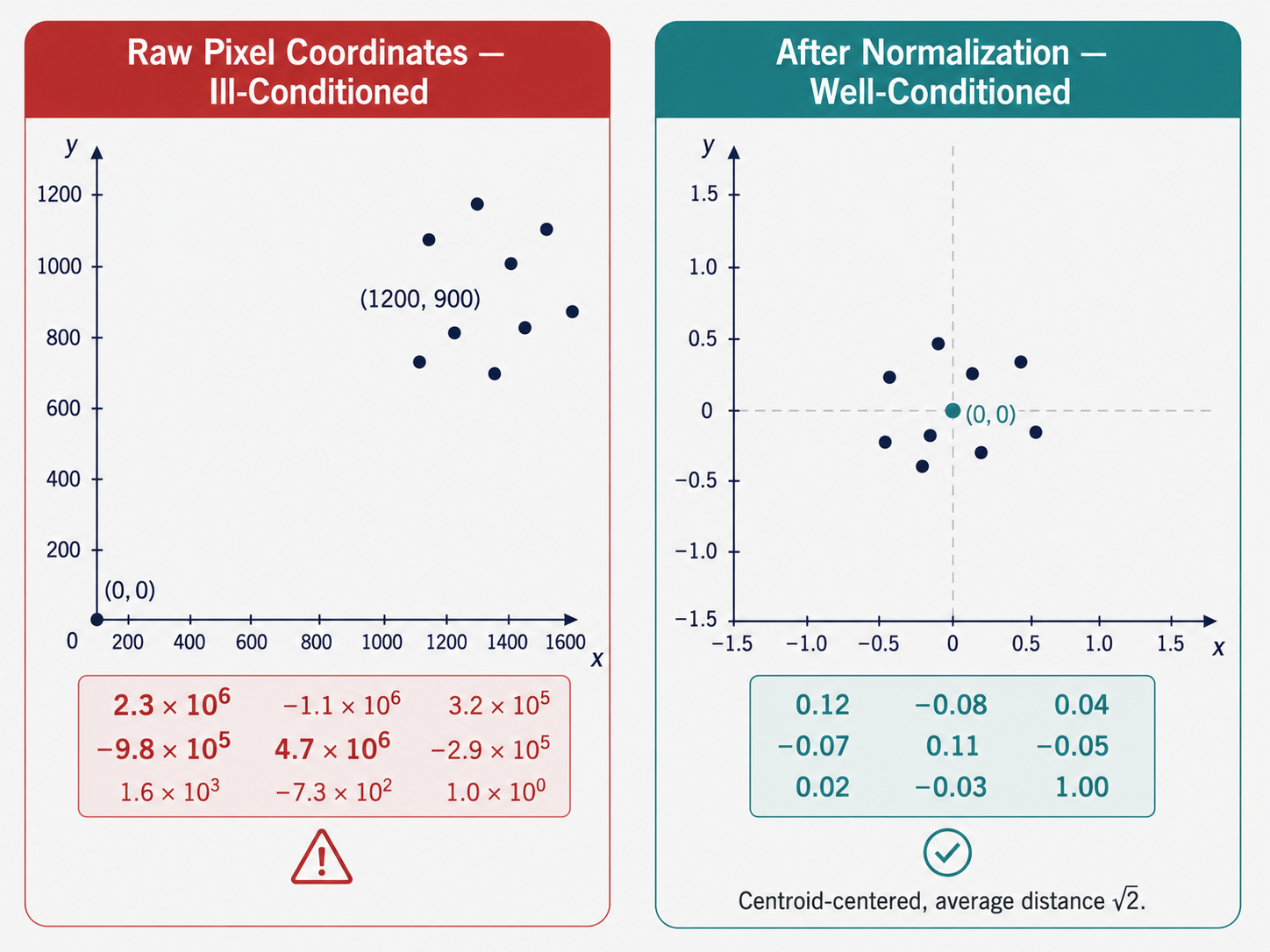
The fix is normalization, introduced by Hartley. Before constructing $W$, we apply a coordinate transformation to each image independently, satisfying two conditions:

Translation: shift the coordinate origin to the centroid of all the image points.
Scaling: rescale so that the average distance from the origin to the points is $\sqrt{2}$ pixels.

These two operations together ensure that the point coordinates are roughly on the order of 1, making $W$ well-conditioned for SVD. The transformation can be represented as a matrix $T$ (and $T’$ for the second image), giving normalized coordinates $q_i = T p_i$ and $q’_i = T’ p’_i$.

We then run the Eight-Point Algorithm on the normalized coordinates to get $F_q$ — the Fundamental matrix for normalized coordinates. Finally, we de-normalize to recover the Fundamental matrix in the original pixel coordinate system:

\[F = T'^T F_q T\]

This normalized version works reliably in practice, reducing the point-to-epipolar-line error from tens of pixels (with the naive version) to sub-pixel accuracy.

Part 5: Image Rectification — Achieving the Ideal Parallel Configuration

Why Rectification Matters

Recall the ideal stereo configuration: two cameras with parallel image planes, where corresponding points share the same row coordinate. In this configuration, stereo matching reduces to a 1D horizontal search. But in practice, two cameras are rarely in this perfect configuration — they might be angled toward each other, tilted, or mounted with slight misalignment.

Image rectification is the process of computing and applying projective transformations (homographies) to both images so that the result looks as if the images were taken by a parallel stereo rig. The epipolar lines become horizontal, and corresponding points end up on the same row.

The Rectification Strategy

The key insight is that the epipoles encode the “badness” of the alignment. In an ideally rectified pair, the epipoles are at infinity along the horizontal axis. So the rectification goal is: find homographies $H_1$ and $H_2$ to apply to the two images such that the epipoles are mapped to horizontal infinity.

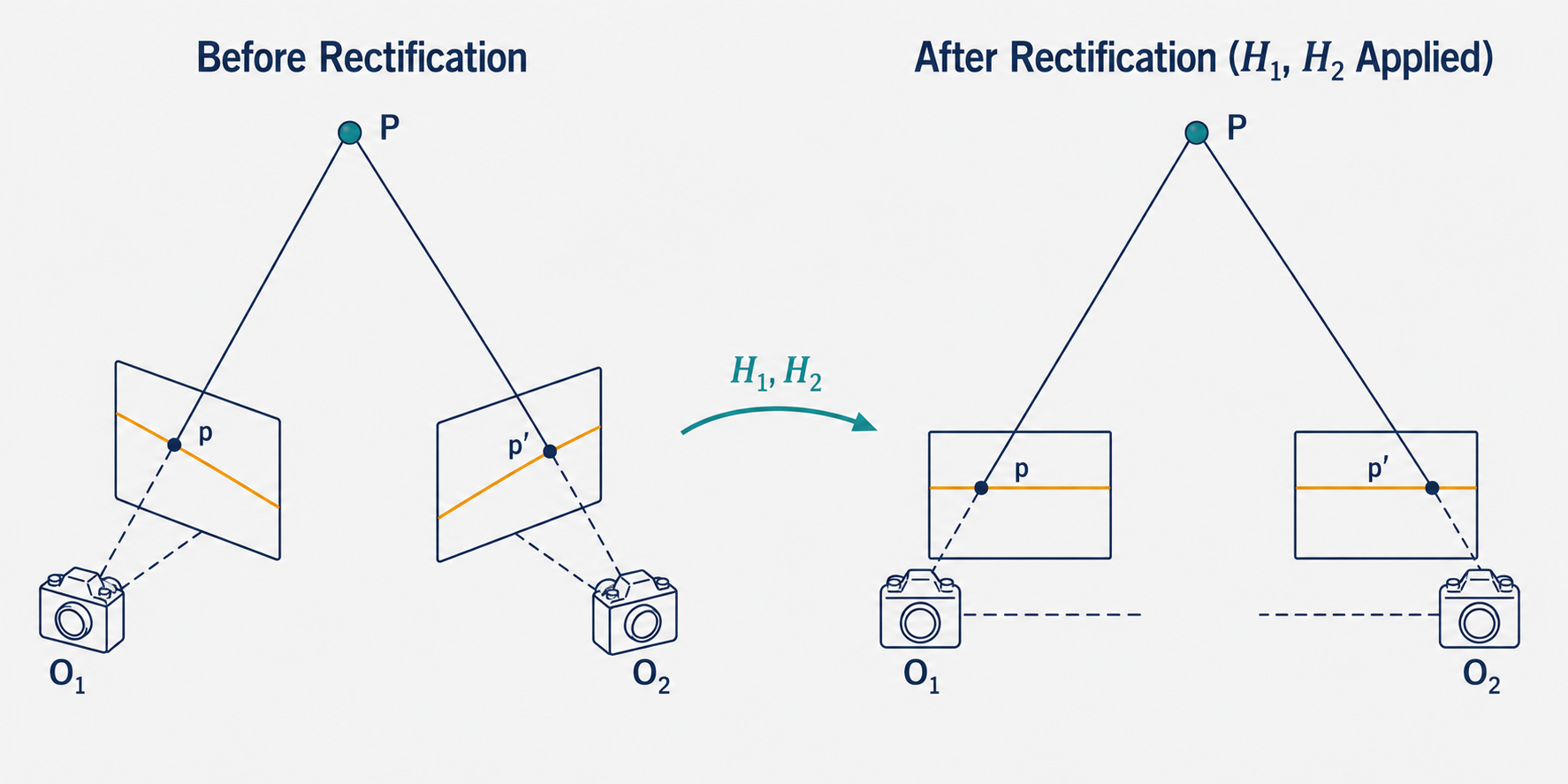
We don’t need to know $K$, $R$, or $T$ to do this. We start from the Fundamental matrix (estimated via the Normalized Eight-Point Algorithm) and the correspondences, and proceed as follows.

Step 1: Find the epipoles. From the Fundamental matrix, we know that each epipolar line $\ell_i = F^T p_i$ passes through the epipole $e’$. In theory, all epipolar lines intersect at $e’$. In practice (due to measurement noise), they don’t all pass through exactly the same point, so we find $e’$ by minimizing the least-squares fitting error — essentially solving the system:

\[\begin{bmatrix} \ell_1^T \\ \vdots \\ \ell_n^T \end{bmatrix} e' = 0\]

via SVD. The epipole $e$ in the first image is found analogously.

Step 2: Construct $H_2$ to rectify the second image. We want to map the epipole $e’$ to a point at infinity on the horizontal axis. This is accomplished through a three-step sequence of transformations:

First, translate the image so its center is at the coordinate origin:

\[T = \begin{bmatrix} 1 & 0 & -\text{width}/2 \\ 0 & 1 & -\text{height}/2 \\ 0 & 0 & 1 \end{bmatrix}\]

Then, rotate to place the translated epipole $Te’$ onto the horizontal axis. If $Te’ = (e’_1, e’_2, 1)$, the rotation is:

\[R = \begin{bmatrix} \alpha \frac{e'_1}{\sqrt{e'^2_1 + e'^2_2}} & \alpha \frac{e'_2}{\sqrt{e'^2_1 + e'^2_2}} & 0 \\ -\alpha \frac{e'_2}{\sqrt{e'^2_1 + e'^2_2}} & \alpha \frac{e'_1}{\sqrt{e'^2_1 + e'^2_2}} & 0 \\ 0 & 0 & 1 \end{bmatrix}\]

where $\alpha = \text{sign}(e’_1)$ ensures the epipole ends up on the positive horizontal axis. After rotation, the epipole is at some finite point $(f, 0, 1)$. To send it to infinity, we apply the projective transformation:

\[G = \begin{bmatrix} 1 & 0 & 0 \\ 0 & 1 & 0 \\ -1/f & 0 & 1 \end{bmatrix}\]

This maps the point $(f, 0, 1)$ to $(f, 0, 0)$ — a point at infinity in the horizontal direction. Finally, translate back:

\[H_2 = T^{-1} G R T\]

Step 3: Construct $H_1$ for the first image. We can’t apply $H_2$ independently to both images — the horizontal alignment of corresponding points would be destroyed. We need $H_1$ to be chosen such that corresponding points $(p_i, p’_i)$ end up on the same row after applying $H_1$ and $H_2$ respectively.

The matching homography has the form:

\[H_1 = H_A H_2 M\]

where $M$ is derived from the Fundamental matrix as $M = [e]_\times F + e v^T$ for some vector $v$ (in practice, $v^T = (1,1,1)$ works well), and $H_A$ is a matrix of the form:

\[H_A = \begin{bmatrix} a_1 & a_2 & a_3 \\ 0 & 1 & 0 \\ 0 & 0 & 1 \end{bmatrix}\]

The three parameters $(a_1, a_2, a_3)$ are found by least-squares. We compute the transformed points $\hat{p}_i = H_2 M p_i$ and $\hat{p}’_i = H_2 p’_i$, and then solve the least-squares problem:

\[\arg\min_a \sum_i (a_1 \hat{x}_i + a_2 \hat{y}_i + a_3 - \hat{x}'_i)^2\]

This is a standard linear least-squares system $Wa = b$, easily solved by standard methods. Once $a$ is found, $H_A$ is determined and $H_1 = H_A H_2 M$ is complete.

The result: applying $H_1$ to the first image and $H_2$ to the second produces a rectified stereo pair where every pair of corresponding points lies on the same horizontal scan line.

Part 6: Conceptual Synthesis — The Full Picture

It is worth stepping back to appreciate the conceptual architecture of what we have built.

The epipolar constraint $p^T F p’ = 0$ is a single bilinear equation relating two image points that depict the same 3D point. It is the fundamental equation of stereo vision. Everything else in this framework is built around computing $F$ (or its calibrated counterpart $E$) and exploiting the constraint it encodes.

The Essential matrix $E$ and Fundamental matrix $F$ are related by the intrinsic camera matrices: $F = K’^{-T} E K^{-1}$. The Essential matrix is the “pure geometry” version, capturing only the relative rotation and translation. The Fundamental matrix is the “complete” version, baking in the cameras’ intrinsics as well. When the cameras are known (calibrated), use $E$; when they’re not, use $F$.

The Eight-Point Algorithm (in its normalized form) is the canonical method for estimating $F$ from scratch. It requires only pixel correspondences — no calibration targets, no known 3D structure, no camera specifications. The geometric information latent in the relative positions of matching features across two images is sufficient to determine the entire epipolar geometry.

Rectification is the practical payoff. By remapping both images into the parallel-camera configuration, we convert the problem of stereo matching — finding corresponding pixels across two arbitrary images — into a structured, efficient 1D search problem. This is the prerequisite for stereo depth estimation, the technology behind autonomous vehicle perception, AR/VR depth sensing, and dense 3D reconstruction from stereo pairs.

There is also a deeper philosophical point here. The Fundamental matrix encodes, in a $3 \times 3$ matrix with 7 degrees of freedom, the entire geometric relationship between two cameras and the scene they observe — without any explicit knowledge of the 3D scene structure. This is a form of structure-from-motion bootstrapping: from the statistics of which pixels in two images match each other, we recover the spatial arrangement of the cameras themselves. Two photographs know things about each other, and about the world that made them, that neither photograph knows alone.

Conclusion: The Geometry of a Stereo Pair

Epipolar geometry is, at its core, the mathematics of having two eyes. It formalizes the intuition that two views of a scene contain vastly more information than the sum of their parts — not because each view is more informative individually, but because the relationship between the views encodes 3D structure.

The epipolar plane, baseline, epipoles, and epipolar lines form a geometric vocabulary that describes how a 3D point’s projections across two cameras are constrained. The Essential matrix makes this constraint algebraic for calibrated cameras; the Fundamental matrix extends it to the uncalibrated case. The Eight-Point Algorithm (especially in its normalized form) gives us a practical and surprisingly clean way to estimate $F$ from raw pixel correspondences. And image rectification translates all this theory into the computationally convenient parallel-camera form that makes stereo matching efficient in practice.

From a single equation — $p^T F p’ = 0$ — flows an entire pipeline capable of calibrating cameras, matching images, localizing objects in 3D space, and reconstructing scenes from scratch. It is a testament to the power of geometric thinking in computer vision, and a reminder that even a pair of flat photographs contains, encoded in the geometry of their pixels, a rich and recoverable model of the three-dimensional world.

This article is based on CS231A Course Notes 3: Epipolar Geometry, by Kenji Hata and Silvio Savarese, Stanford University.

Epipolar Geometry