Finding Structure in Noise: A Deep Dive into Fitting and Matching

Finding Structure in Noise: A Deep Dive into Fitting and Matching

From least squares to RANSAC to the Hough transform — how computer vision algorithms find clean geometric structure hidden inside messy, real-world data.

Introduction: The Universal Problem of Finding Patterns

Every time a self-driving car detects a lane boundary, or a panorama app stitches two photos together, or a robot arm identifies an object to pick up, the same fundamental challenge arises: how do you find a clean, structured model inside data that is noisy, imprecise, and full of distractions?

This is the fitting problem. You have a set of observed data points, and you want to find the parameters of a geometric model — a line, a plane, a homography, a fundamental matrix — that best explains what you see. The data will never be perfect. Real measurements are noisy. Sensors make errors. And often, a significant fraction of your data points are outliers — observations that are simply wrong, resulting from sensor glitches, misidentified features, or spurious detections that have nothing to do with the structure you are trying to find.

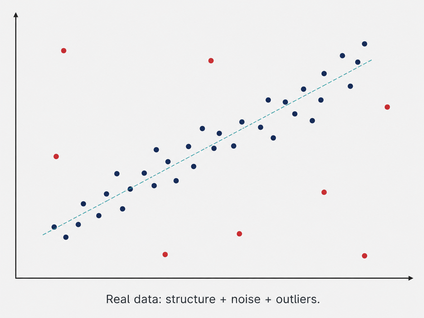
The difference between a working vision system and a broken one often comes down entirely to how well it handles this fitting problem. A method that crumbles in the presence of outliers is not a method you can deploy in the real world. The story of fitting in computer vision is a story of progressively smarter strategies for dealing with the messy reality of data.

In this article, we will develop three major fitting strategies from the ground up: least squares (the classical approach, powerful but fragile), RANSAC (a randomized method that is remarkably robust), and the Hough transform (a clever change of perspective that turns fitting into a voting problem). Each solves a different piece of the puzzle, and together they form a toolkit that appears throughout modern computer vision.

Part 1: Least Squares — The Classical Foundation

What Are We Trying to Do?

Let us begin with the simplest instantiation of the fitting problem: fitting a line to a set of 2D points.

You have $N$ data points ${(x_i, y_i)}_{i=1}^N$ that approximately lie along a straight line, but not perfectly — each point is displaced from the true line by some small amount of noise. You want to find the line parameters that give the best fit.

The naive approach would be to find a line that passes exactly through some of the points, but this ignores most of the data and is extremely sensitive to which specific points you choose. The principled approach is to use all the data simultaneously, defining a global measure of goodness-of-fit and minimizing it.

Ordinary Least Squares: Minimizing Vertical Errors

The most classical fitting criterion is least squares. For a line $y = mx + b$, the model prediction for input $x_i$ is $\hat{y}_i = mx_i + b$. The residual for point $i$ is the difference between the observed $y_i$ and the predicted $\hat{y}_i$:

\[r_i = y_i - \hat{y}_i = y_i - mx_i - b\]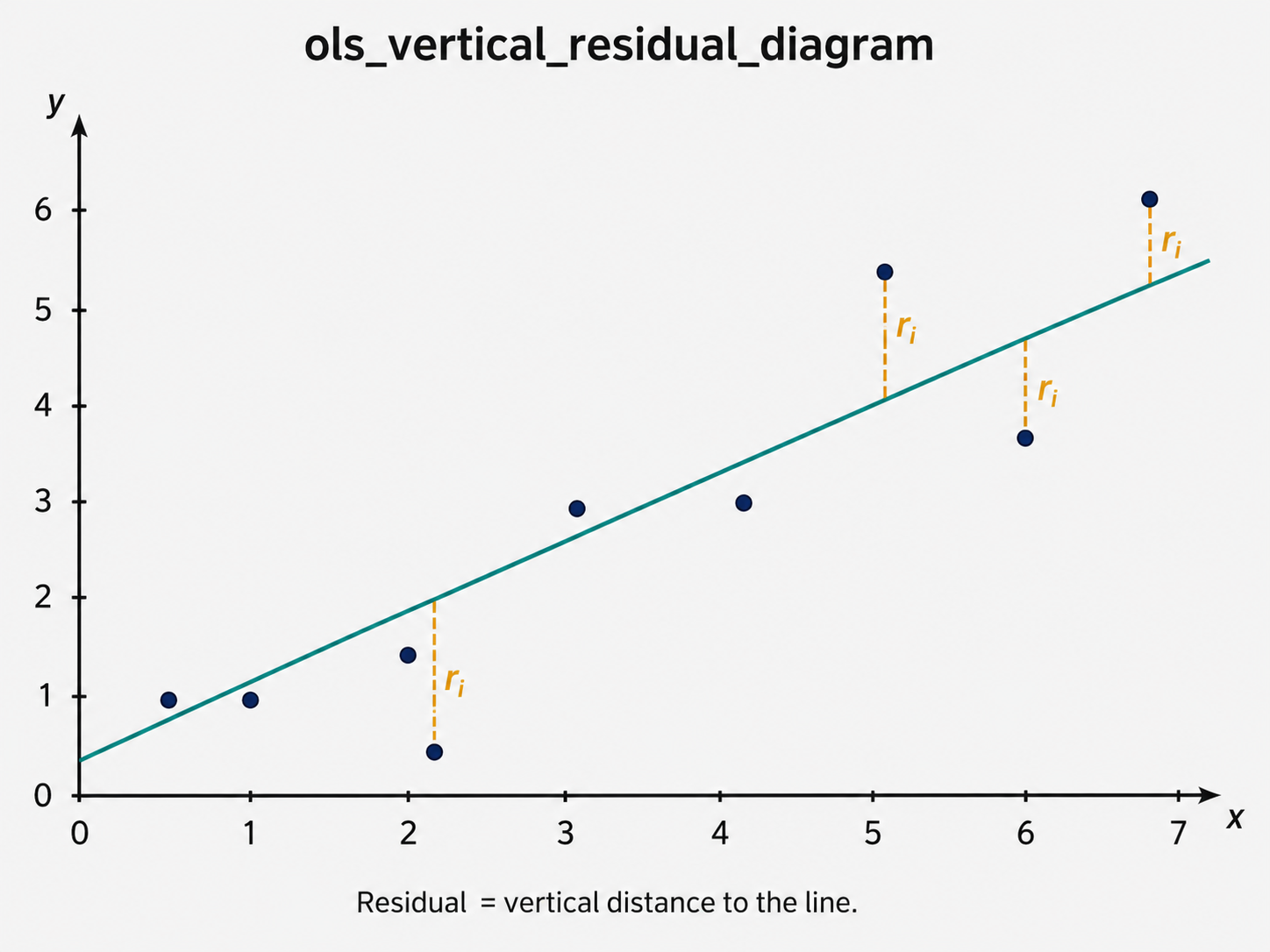

Least squares finds the parameters $m$ and $b$ that minimize the total squared residual:

\[E = \sum_{i=1}^{N} (y_i - mx_i - b)^2\]

Squaring the residuals serves two purposes: it makes the criterion differentiable (allowing calculus-based optimization), and it ensures that positive and negative errors do not cancel each other out. It also has a deeper statistical justification — it is the maximum likelihood estimator when the noise on each observation is independent and Gaussian.

Deriving the Solution

The power of least squares is that it has a closed-form solution — no iteration required, just a matrix inversion. To see why, rewrite the error in compact matrix notation.

Define the vector of observations $\mathbf{y} = [y_1, \ldots, y_N]^T$, the parameter vector $\mathbf{w} = [m, b]^T$, and the design matrix:

\[X = \begin{pmatrix} x_1 & 1 \\ x_2 & 1 \\ \vdots & \vdots \\ x_N & 1 \end{pmatrix}\]

Then the error becomes $E = |\mathbf{y} - X\mathbf{w}|^2$. Expanding and taking the gradient with respect to $\mathbf{w}$:

\[\nabla_\mathbf{w} \|\mathbf{y} - X\mathbf{w}\|^2 = -2X^T\mathbf{y} + 2X^TX\mathbf{w}\]

Setting this equal to zero yields the famous normal equations:

\[X^TX\mathbf{w} = X^T\mathbf{y}\]

When $X$ has full column rank — meaning no two rows are proportional — the matrix $X^TX$ is invertible, and the solution is:

\[\mathbf{w} = (X^TX)^{-1}X^T\mathbf{y}\]

The quantity $(X^TX)^{-1}X^T$ is called the Moore-Penrose pseudoinverse of $X$, often written $X^+$. It appears throughout linear algebra as the go-to tool for solving overdetermined systems (more equations than unknowns) in the least-squares sense.

The Problem with Vertical Lines: Moving to Total Least Squares

The formulation above measures errors only in the vertical ($y$) direction. The residual $y_i - \hat{y}_i$ asks: “how far is the point from the line in the $y$-direction?” This is asymmetric — it treats $x$ as an exact independent variable and $y$ as the noisy one.

This asymmetry causes a practical disaster: the method completely fails for vertical or near-vertical lines. If the true line is nearly vertical, the slope $m$ becomes enormous (or technically undefined for a perfectly vertical line), leading to numerical instability.

The fix is to switch to a symmetric line parameterization: $ax + by + c = 0$, where the vector $\vec{n} = (a, b)$ is the normal to the line. This form can represent lines of any orientation, including vertical (just set $b = 0$).

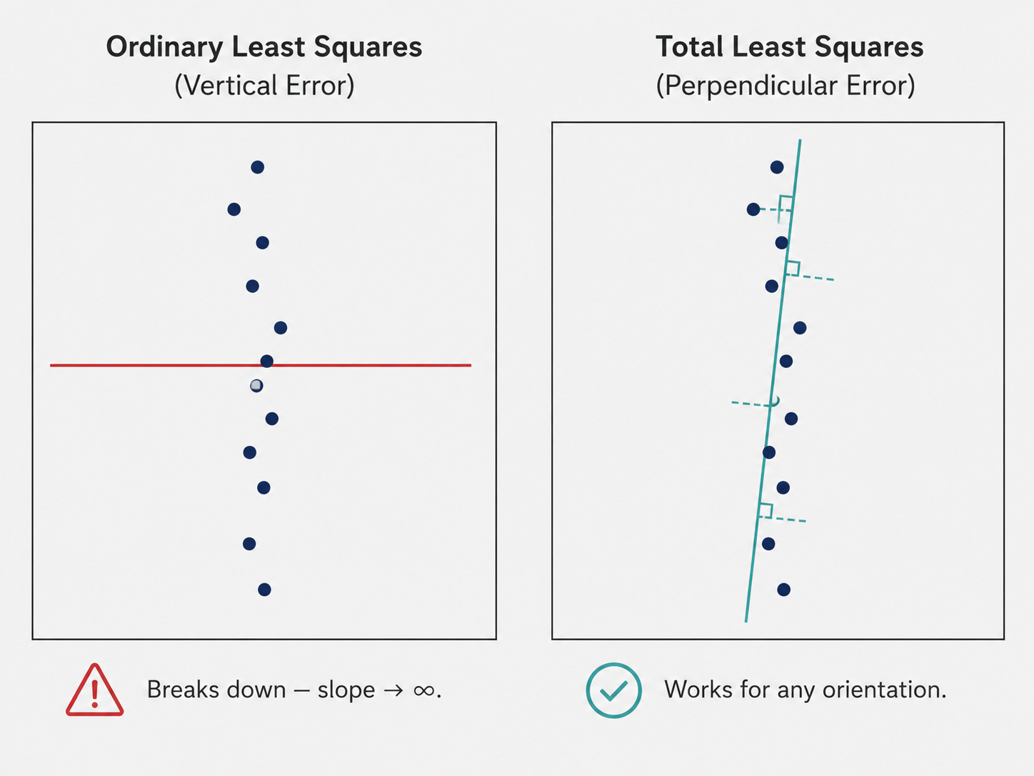
In this parameterization, the distance from a point $(x_i, y_i)$ to the line is the perpendicular distance — the shortest possible distance, measured at right angles to the line. This is given by:

\[d_i = \frac{|ax_i + by_i + c|}{\sqrt{a^2 + b^2}}\]

The proof is simple. The distance from a point $P = (x_i, y_i)$ to a line $ax + by + c = 0$ is the length of the vector from $P$ to its nearest point $Q$ on the line, which is the component of $\overrightarrow{QP}$ along the unit normal $\hat{n} = (a,b)/|(a,b)|$. Working through the dot product gives exactly the formula above.

The new error criterion — total least squares — minimizes the sum of squared perpendicular distances:

\[E = \sum_{i=1}^{N} (ax_i + by_i + c)^2 \quad \text{subject to } a^2 + b^2 = 1\]

The constraint $a^2 + b^2 = 1$ normalizes the line, ensuring the distance formula is valid and making the solution unique up to sign.

Solving Total Least Squares via SVD

Solving the constrained total least squares problem requires a bit more elegance than ordinary least squares. The key insight is that the optimal line must pass through the centroid of the data, $(\bar{x}, \bar{y})$.

To see why, notice that the error $E$ can be decomposed using the Pythagorean theorem. Any candidate line passing through a point $(x_0, y_0)$ other than the centroid can be improved by shifting it to pass through the centroid instead — the shifted line always reduces the total error. This can be shown rigorously: defining the residuals around an arbitrary center $(x_0, y_0)$ versus the centroid, one obtains $E(a, b, x_0, y_0) \geq E(a, b, \bar{x}, \bar{y})$ with equality only when $(x_0, y_0)$ is the centroid.

With the constraint that the line passes through $(\bar{x}, \bar{y})$, we can eliminate $c$ by substituting $c = -a\bar{x} - b\bar{y}$, and center the data by computing $\tilde{x}_i = x_i - \bar{x}$, $\tilde{y}_i = y_i - \bar{y}$. The error simplifies to:

\[E = \left\| \begin{pmatrix} \tilde{x}_1 & \tilde{y}_1 \\ \vdots & \vdots \\ \tilde{x}_N & \tilde{y}_N \end{pmatrix} \begin{pmatrix} a \\ b \end{pmatrix} \right\|^2 = \|X\mathbf{w}\|^2 \quad \text{subject to } \|\mathbf{w}\|^2 = 1\]

This is a classic constrained least-norm problem: minimize $|X\mathbf{w}|^2$ subject to $|\mathbf{w}|^2 = 1$. The solution comes directly from the Singular Value Decomposition (SVD) of $X = U \Sigma V^T$.

To minimize $|X\mathbf{w}|^2 = |\Sigma V^T \mathbf{w}|^2$ (using the fact that $U$ is orthonormal and preserves norms), set $\mathbf{v} = V^T\mathbf{w}$. The problem becomes minimizing $|\Sigma \mathbf{v}|^2$ subject to $|\mathbf{v}|^2 = 1$. The diagonal matrix $\Sigma$ scales each component of $\mathbf{v}$ by the corresponding singular value $\sigma_i$. To minimize the result, point $\mathbf{v}$ entirely in the direction of the smallest singular value — i.e., $\mathbf{v} = [0, 1]^T$ (the last standard basis vector, since singular values are sorted in descending order).

Recovering $\mathbf{w} = V\mathbf{v}$ gives: the optimal line normal is the last column of $V$ in the SVD of the centered data matrix. This elegant result says that total least squares finds the direction of minimum variance in the data — the direction along which the data varies least, which is perpendicular to the best-fit line.

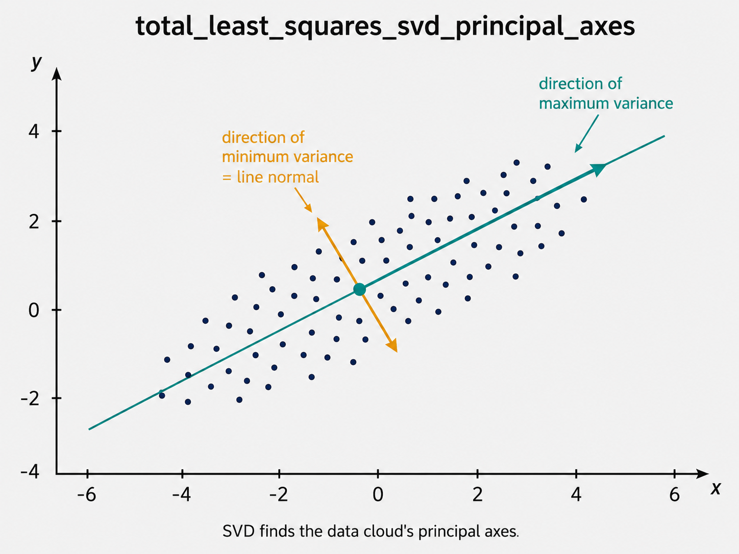
This SVD interpretation has a beautiful geometric meaning: SVD finds the principal axes of the data cloud, and total least squares picks the axis of least spread as the line normal.

Why Least Squares Breaks Down: The Outlier Problem

Both ordinary and total least squares share a critical vulnerability: outliers. An outlier is a data point that lies far from the true structure — perhaps due to a sensor glitch, a misidentified feature match, or a measurement from a completely different structure in the scene.

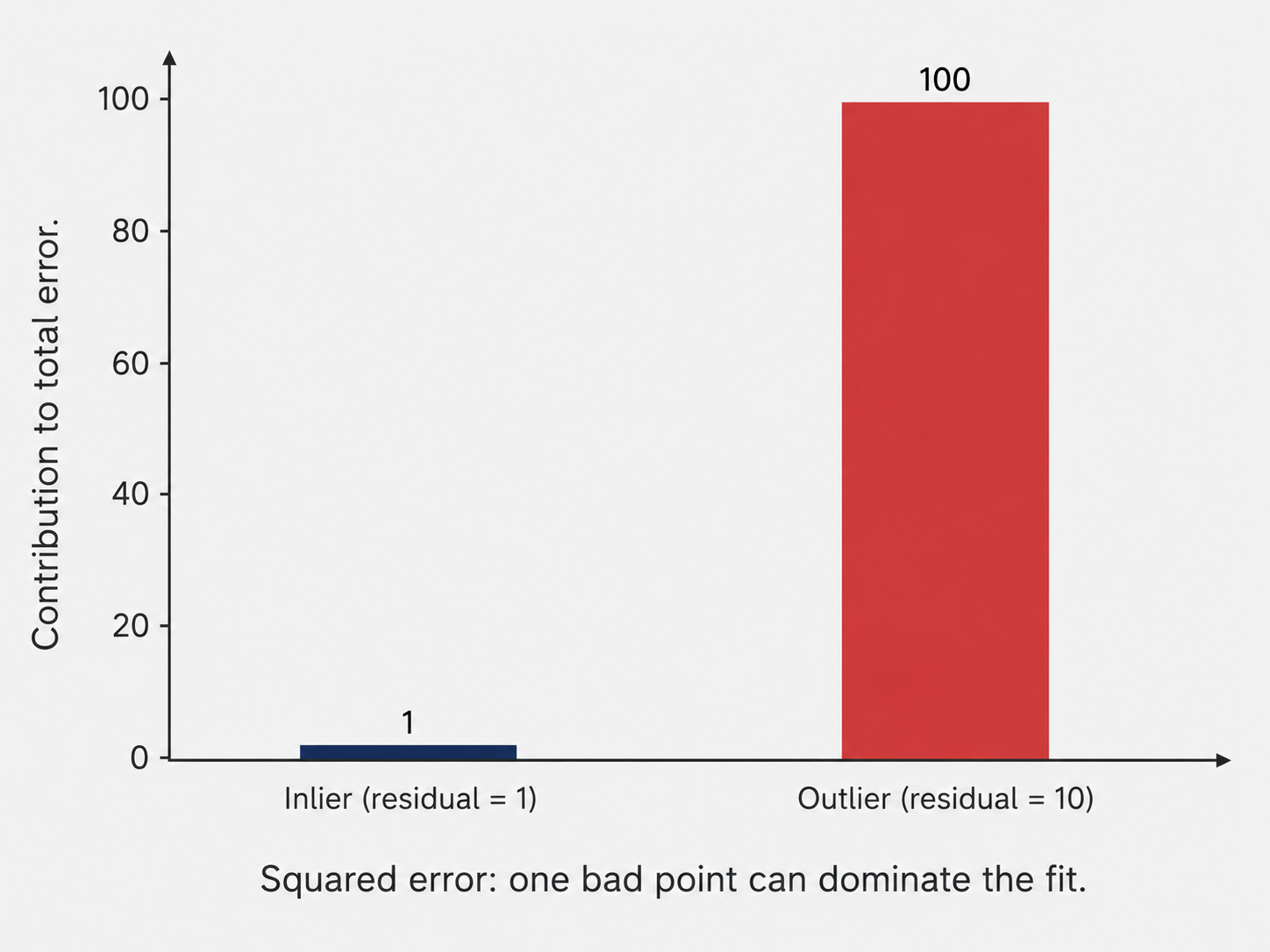
The quadratic error $C(u_i) = u_i^2$ means that an outlier with residual $u_i = 10$ contributes $100$ to the error, while a typical inlier with residual $u_i = 1$ contributes only $1$. The outlier’s contribution is a hundred times larger. In minimizing the total error, the algorithm devotes enormous effort to satisfying the outlier, pulling the fitted model away from the majority of correct points. One bad point can ruin everything.

A natural response is to use a robust cost function that grows more slowly for large residuals. One example is:

\[C(u_i, \sigma) = \frac{u_i^2}{\sigma^2 + u_i^2}\]

When $u_i$ is small (inlier), $C \approx u_i^2 / \sigma^2$ — this behaves like squared error, penalizing deviations from the model. When $u_i$ is large (outlier), $C \to 1$ — the cost saturates, capping the damage any single outlier can do.

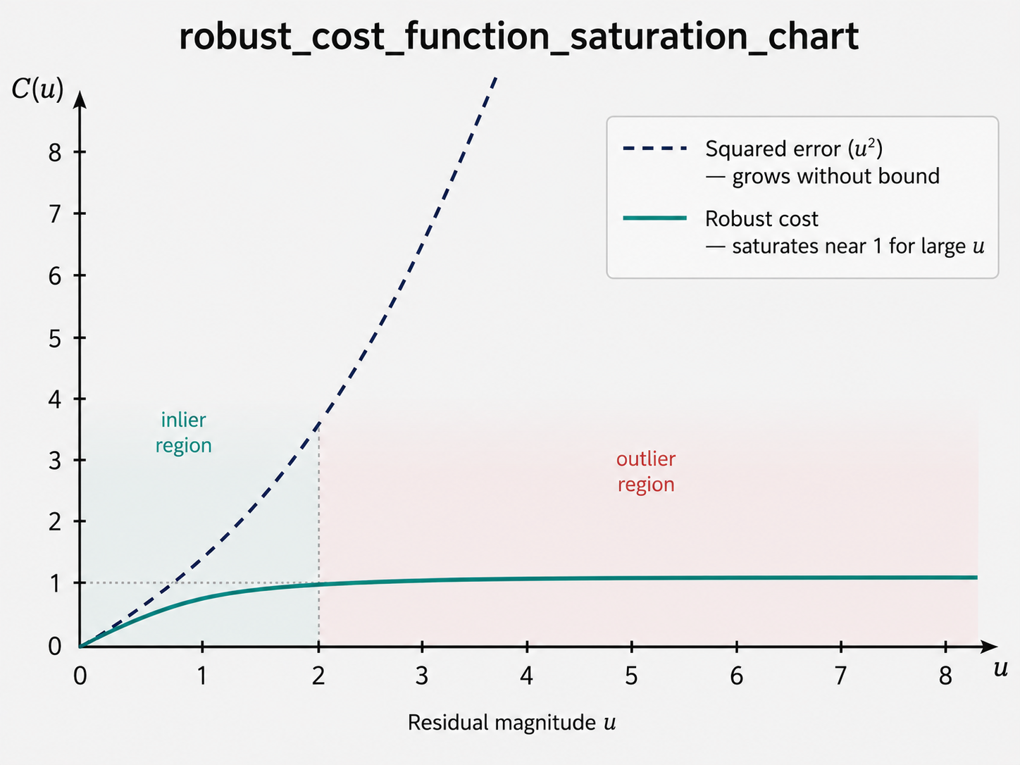
The parameter $\sigma$ — the scale parameter — controls the transition between “treated as inlier” and “treated as outlier.” A large $\sigma$ behaves nearly like standard least squares. A small $\sigma$ treats almost everything as an outlier and fits only the very closest points. Choosing $\sigma$ well is essential but non-trivial; it typically requires some knowledge of the noise scale.

Because robust cost functions are nonlinear, they cannot be minimized in closed form. Instead, the standard approach is to start with the least-squares solution as initialization, then iteratively minimize the robust objective using gradient-based methods until convergence.

Part 2: RANSAC — Robust Fitting Through Random Sampling

A Different Philosophy Entirely

Robust cost functions approach the outlier problem by down-weighting suspicious points. RANSAC — RAndom SAmple Consensus — takes a completely different approach: rather than trying to fit all the data while mitigating outlier influence, it finds the subset of the data that is most consistent with some model and fits only that subset.

The intuition is powerful and practical. If you have 100 data points and 40 are outliers, there exists a large “inlier set” of 60 points that all agree on the same underlying model. If you could identify which points belong to the inlier set, standard least squares on those 60 points would give an excellent fit. The challenge is finding that inlier set without knowing the model, and finding the model without knowing the inlier set. RANSAC breaks this circularity with a randomized approach.

The Algorithm

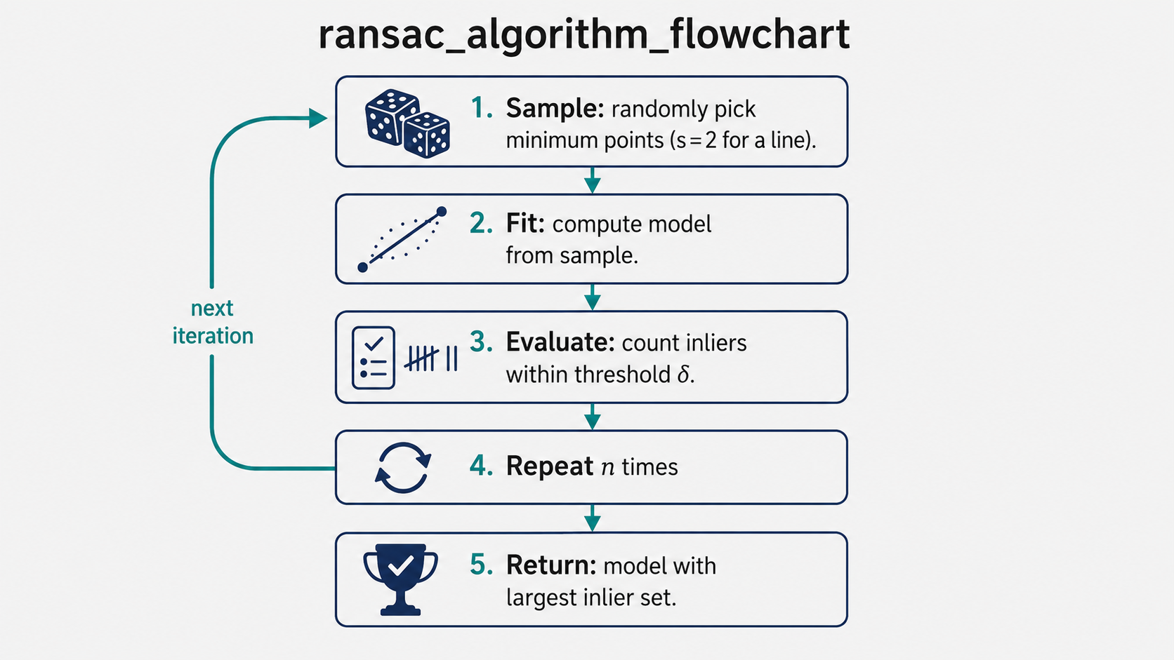
RANSAC for line fitting works as follows. Suppose we have $N$ points that we believe mostly lie along a single line, with some outliers scattered randomly.

Step 1 — Sample: Randomly choose the minimum number of points needed to define the model. For a line, this is exactly 2 points. (For a homography, it would be 4 point correspondences. For a fundamental matrix, it would be 8.)

Step 2 — Fit: Fit the model to the sampled points. For two points, there is exactly one line through them.

Step 3 — Evaluate: Count the inliers — all data points within a distance threshold $\delta$ of the fitted model. Formally, the inlier set is: $P = \{(x_i, y_i) \mid r((x_i, y_i), \mathbf{w}) < \delta\}$ where $r$ is the residual (perpendicular distance to the line) and $\delta$ is a pre-chosen tolerance. The outlier set is simply everything not in $P$.

Step 4 — Repeat: Go back to Step 1 with a new random sample. Do this for $n$ iterations.

Step 5 — Return: Return the model corresponding to the largest inlier set found across all iterations. Optionally, refit the model using least squares on the entire final inlier set for a more accurate estimate.

Think of RANSAC like a detective canvassing witnesses. Rather than trying to extract a story that reconciles every account (including the unreliable ones), the detective finds the largest group of witnesses whose stories are mutually consistent, and builds the case from those.

How Many Iterations Do You Need?

The key question is: how many iterations $n$ are sufficient to be confident that at least one of your random samples contains only inliers?

Let $\epsilon \in [0, 1]$ be the fraction of outliers in the data, and let $s$ be the minimum sample size (for a line, $s = 2$). The probability that a single randomly drawn sample of size $s$ contains all inliers is:

\[(1 - \epsilon)^s\]

The probability that a single sample contains at least one outlier is:

\[1 - (1 - \epsilon)^s\]

The probability that all $n$ samples contain at least one outlier (i.e., we never get a clean sample) is:

\[\left(1 - (1 - \epsilon)^s\right)^n\]

So the probability that at least one of the $n$ samples is clean is:

\[p = 1 - \left(1 - (1 - \epsilon)^s\right)^n\]

Solving for $n$ to achieve a desired success probability $p$:

\[n = \frac{\log(1 - p)}{\log\left(1 - (1 - \epsilon)^s\right)}\]

This is a crucial formula. Let us build intuition with some numbers. If 50% of your data are outliers ($\epsilon = 0.5$), fitting a line ($s = 2$), and you want 99% confidence ($p = 0.99$):

\[n = \frac{\log(0.01)}{\log(1 - 0.25)} = \frac{-4.605}{-0.288} \approx 16\]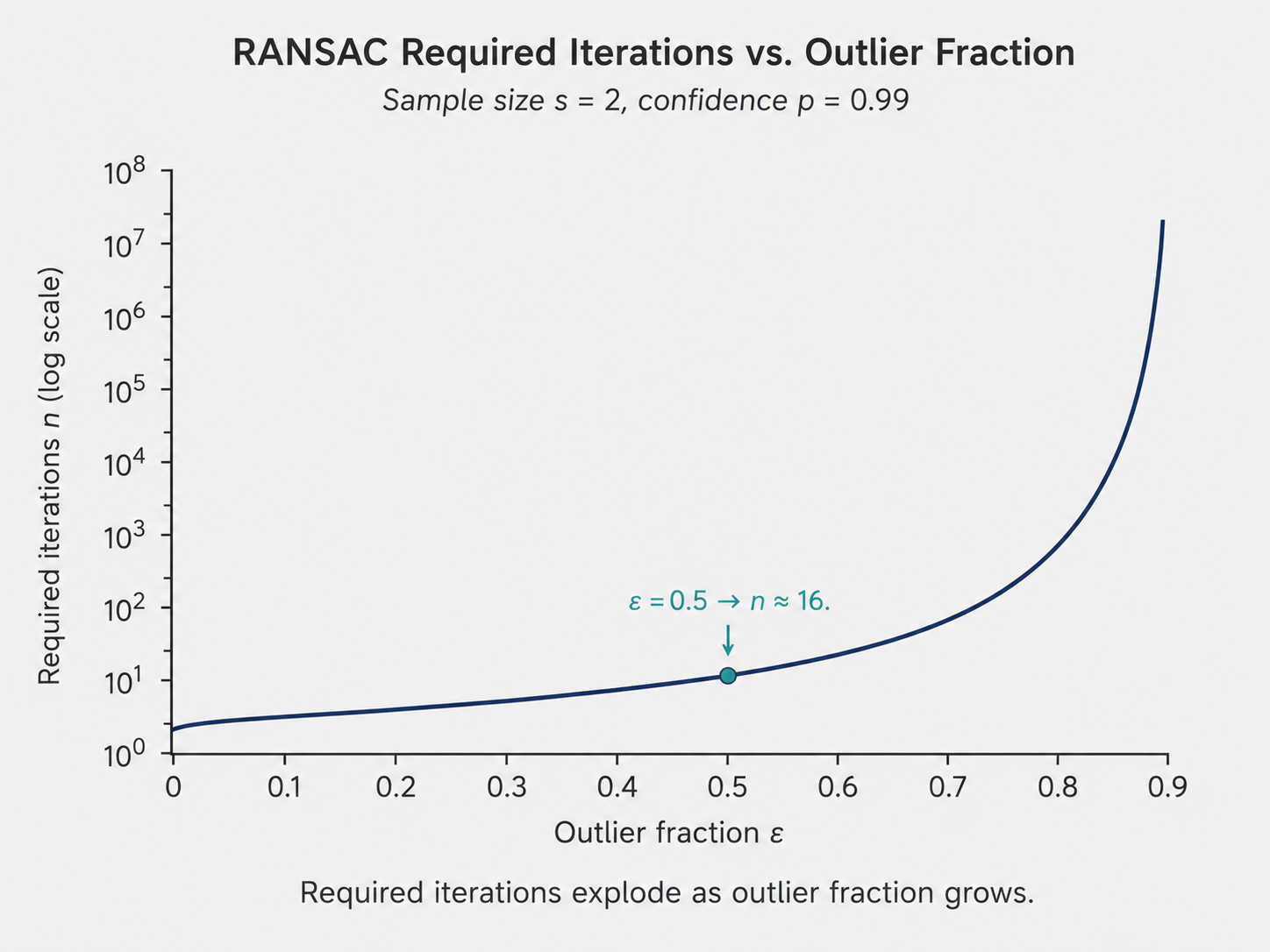

Just 16 iterations are sufficient! RANSAC is remarkably efficient because even with many outliers, the probability of drawing a clean small sample in repeated trials grows quickly. The formula also reveals when RANSAC becomes expensive: when the model requires a large minimum sample size $s$, or when the outlier fraction $\epsilon$ is very high, the required $n$ grows rapidly.

What Makes RANSAC Special

RANSAC has a combination of properties that make it uniquely suited to computer vision:

It is general — the same algorithm structure applies to any parametric model. Change the sampling step and the fitting step, and you have RANSAC for homographies, fundamental matrices, circles, planes, or any other geometric model. In practice, RANSAC is the standard preprocessing step before computing homographies or fundamental matrices from feature point matches, precisely because the matches always contain false matches (outliers) that would corrupt standard least squares.

It is interpretable — after running RANSAC, you have an explicit inlier set and an explicit outlier set. You know which points the algorithm believes are consistent with the model, and which are not. This transparency is valuable in debugging and analysis.

It is robust to high outlier rates — as long as there is a sufficiently large inlier set, RANSAC will find it even when outliers dominate the data.

The main limitations are that $\delta$ (the inlier threshold) and $n$ (the iteration count) need to be specified, RANSAC is probabilistic (there is always a small chance of failure), and when outlier rates are extreme (above roughly 80-90%), the required iteration count explodes.

Part 3: The Hough Transform — Voting in Parameter Space

A Completely Different Way of Thinking About Fitting

Both least squares and RANSAC work by proposing a model and checking how many points agree with it. The Hough transform takes yet another approach — it is fundamentally a voting procedure, and it expresses a profound duality between image space and parameter space.

The core insight is this: rather than asking “what line fits these points?”, flip the question around and ask “what lines are consistent with each individual point?” Each point has an opinion about all possible lines that could pass through it. If you let every point vote for all lines it is consistent with, then the line that the most points agree on will accumulate the most votes. That line is your answer.

The Image-to-Parameter Duality

Let us make this precise for lines of the form $y = mx + n$ (using $n$ for the intercept to avoid confusion with the iteration count).

A single point $(x_i, y_i)$ in image space lies on every line $y = mx + n$ satisfying $y_i = m x_i + n$, or equivalently:

\[n = -x_i m + y_i\]

This is a line in parameter space $(m, n)$ — a linear relationship between the possible slope $m$ and intercept $n$ values. Every $(m, n)$ pair on this line in parameter space corresponds to a line $y = mx + n$ in image space that passes through $(x_i, y_i)$.

Now consider two image points $(x_1, y_1)$ and $(x_2, y_2)$. Each maps to a line in parameter space. If these two points lie on the same image line with parameters $(m’, n’)$, then both parameter-space lines pass through the same point $(m’, n’)$. In other words, the two lines in parameter space intersect at the parameters of the true fitting line.

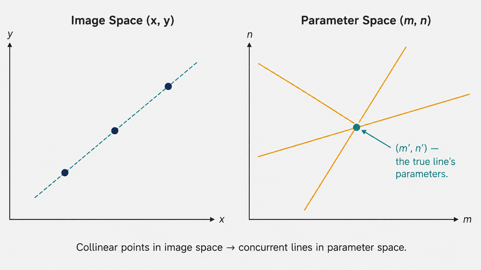
This is the central magic of the Hough transform: collinear points in image space become concurrent lines in parameter space. Finding a line that fits many points is equivalent to finding a point in parameter space where many lines intersect — a peak in a 2D accumulator.

The Practical Algorithm

In practice, the Hough voting procedure works as follows:

Divide the parameter space into a discrete grid of cells, each cell corresponding to a range of $(m, n)$ values. Initialize all cell counts to zero.
For each data point $(x_i, y_i)$, compute all parameter-space cells $(m, n)$ that satisfy $n = -x_im + y_i$ (approximately, snapping to the nearest grid cell), and increment each such cell by 1.
After processing all data points, find the cell with the highest count. The corresponding $(m, n)$ values are the parameters of the best-fit line.

Each point contributes at most one vote per candidate line — hence the “voting” interpretation. Points that lie near a true line will vote heavily for the corresponding parameter-space cell. Random outliers will spread their votes diffusely across many cells, never concentrating enough to form a peak.

One attractive property of the Hough transform is that it naturally handles multiple structures in the data. If the scene contains two lines, there will be two peaks in parameter space. Each peak corresponds to one line, and the votes for each peak come from the points on that line. This is something standard least squares fundamentally cannot do — it fits a single model to everything. RANSAC can handle multiple structures by running sequentially (fit one model, remove its inliers, repeat), but the Hough transform detects all of them simultaneously.

The Problem with Slope-Intercept Parameters: Unbounded Space

There is a significant practical problem with using $(m, n)$ as the parameter space: the slope $m$ is unbounded. A nearly vertical line has $m \to \pm\infty$, making it impossible to allocate a finite grid. This is the same problem we encountered with ordinary least squares.

The solution is to switch to the polar parameterization of lines:

\[x\cos(\theta) + y\sin(\theta) = \rho\]

In this representation:

$\rho$ is the perpendicular distance from the origin to the line — bounded by the maximum distance between any two points in the dataset, which for an image of width $W$ and height $H$ is at most $\sqrt{W^2 + H^2}$.
$\theta$ is the angle of the line’s normal vector with respect to the $x$-axis — bounded in $[0, \pi)$.

Both parameters are finite, so the parameter space grid is finite. Every line, regardless of orientation, is representable.

With the polar parameterization, a single image point $(x_i, y_i)$ corresponds not to a straight line in parameter space, but to a sinusoidal curve:

\[\rho = x_i \cos(\theta) + y_i \sin(\theta)\]

For different values of $\theta$, this traces out a sinusoid in the $(\theta, \rho)$ plane. Collinear image points produce sinusoids that all pass through the same $(\theta, \rho)$ point — the intersection corresponds to the parameters of the common line.

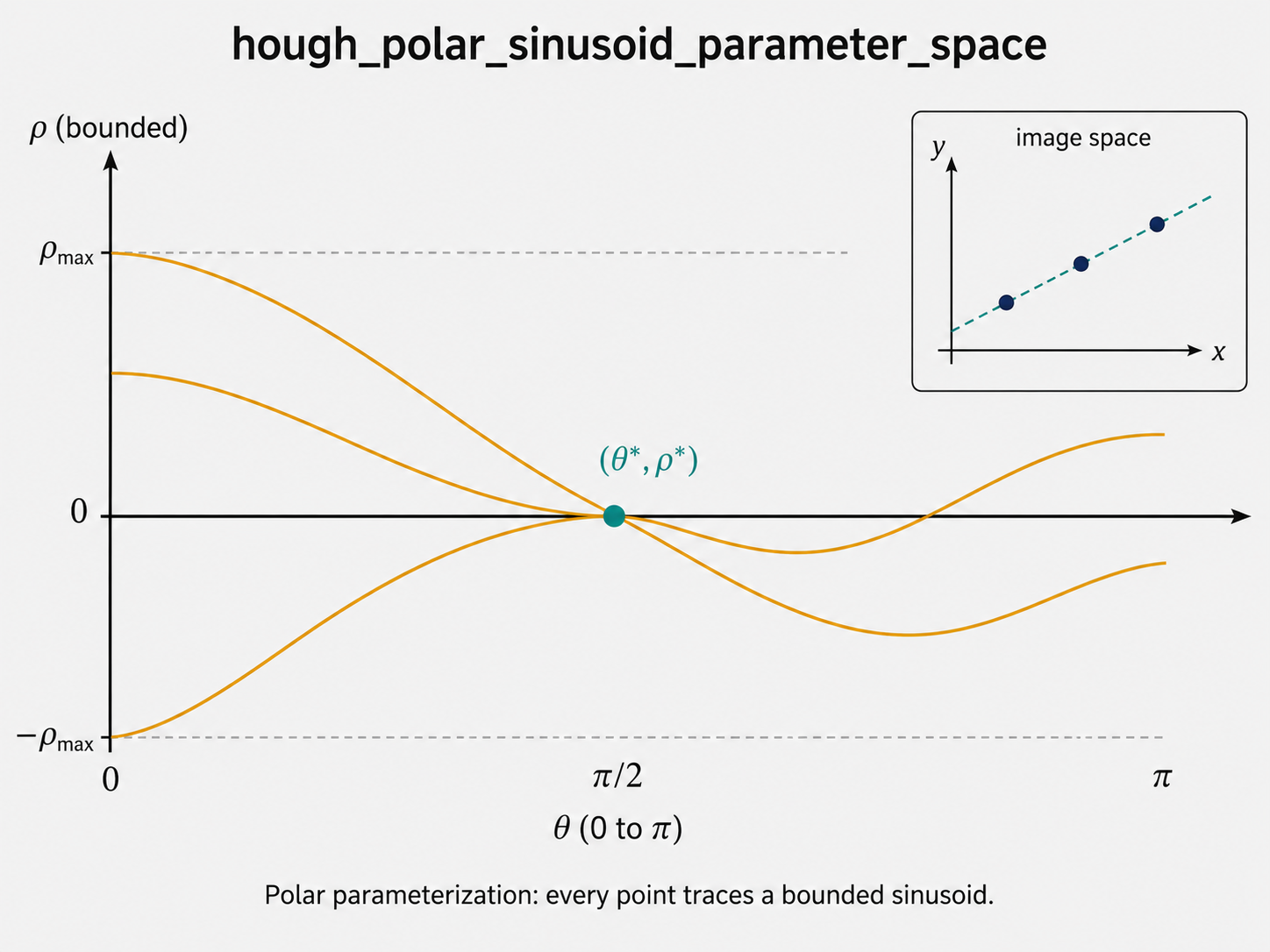
The voting procedure is otherwise identical: for each data point, trace the sinusoid in the $(\theta, \rho)$ grid and increment all touched cells; after processing all points, find the peak.

Handling Noise and Choosing Grid Resolution

A key practical parameter in the Hough transform is the grid cell size $w$. Noisy data points that theoretically should lie on the same line will, in practice, trace sinusoids that do not intersect at exactly one point but rather form a small cluster of nearby intersections. A grid cell that is too fine will have these votes scattered across several cells, producing no clear peak. A coarser grid bins these nearby votes together, producing a clean peak.

But coarser grids introduce their own problem: cells that are too large will merge the votes of two genuinely different nearby lines, blurring them into a single broad peak and losing the ability to distinguish the lines. This is the classical resolution-precision trade-off: fine grids give precise answers but are sensitive to noise; coarse grids tolerate noise but lose precision.

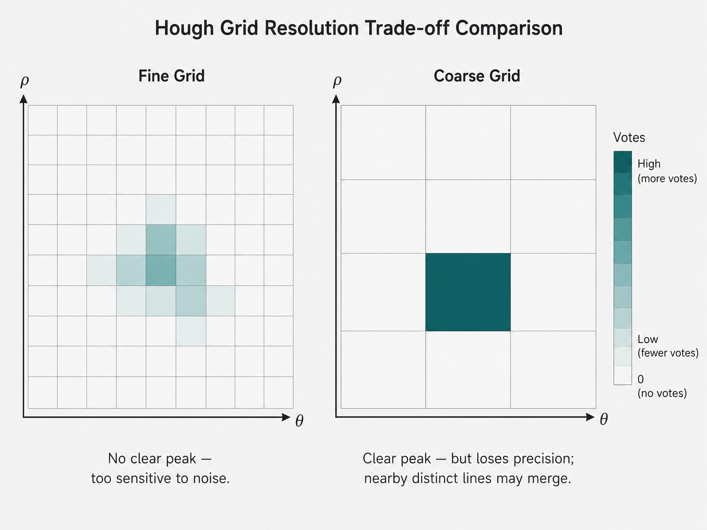
In the presence of truly uniform noise — points scattered randomly everywhere with no underlying structure — the Hough space will be covered with spurious peaks of roughly equal height, and no single candidate line will achieve a decisive majority. The Hough transform, like all fitting methods, requires that the signal-to-noise ratio be sufficient for the structure to be detectable.

Putting It All Together: When to Use Which Method

These three fitting strategies are not competing alternatives — they are complementary tools, each suited to different conditions.

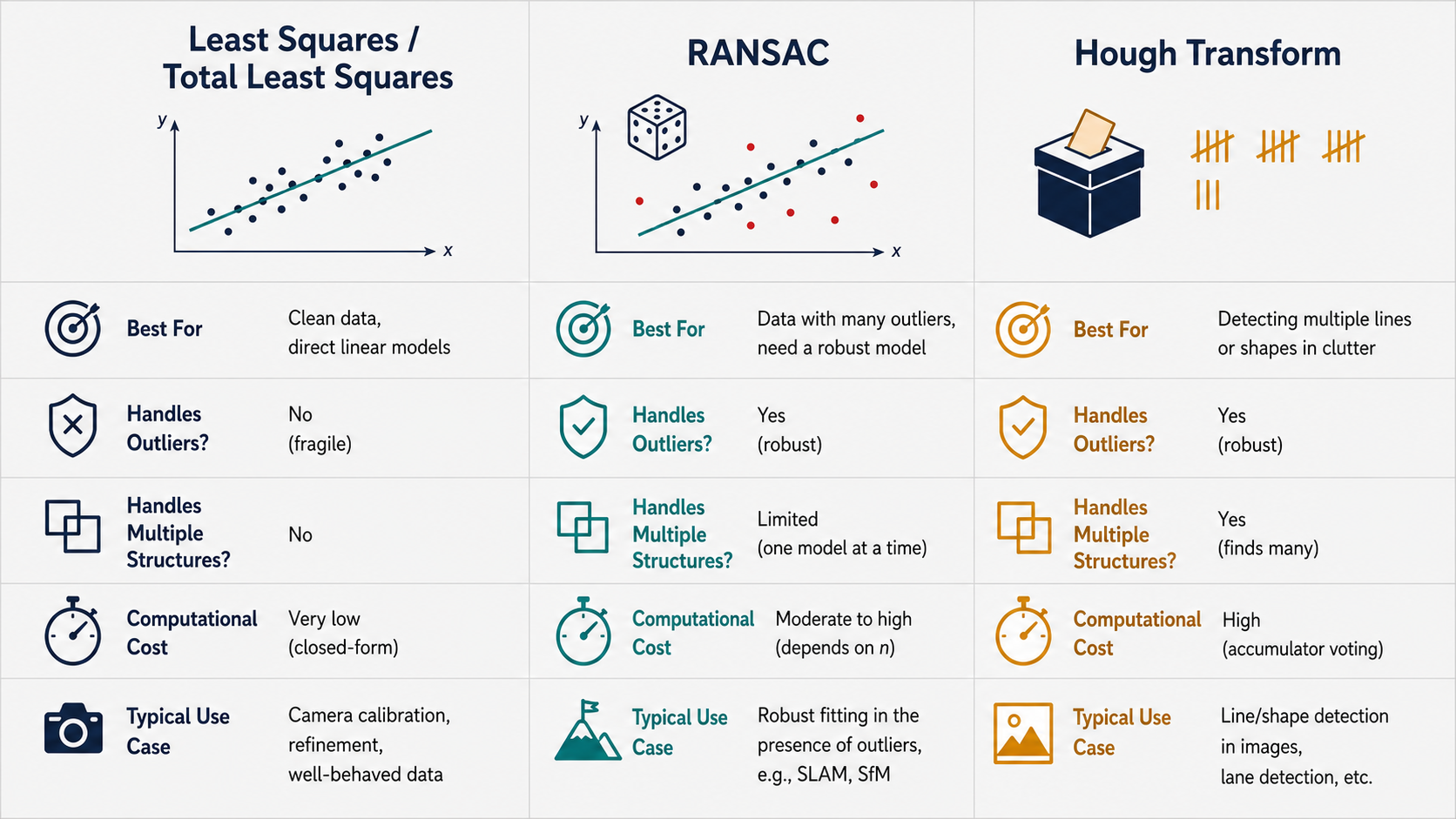
Ordinary least squares is the right starting point when your data is relatively clean and you have a direct, linear parameterization of the model. It is fast, produces a unique solution, and has a beautiful closed-form expression. It is the backbone of camera calibration, homography computation, and fundamental matrix estimation — but always in combination with a robustification step.

Total least squares with SVD is needed when the error should be measured symmetrically (e.g., fitting lines, planes, or subspaces), or whenever the minimum-norm solution to an underdetermined system is needed. The SVD solution appears throughout computer vision: PCA for dimensionality reduction, the eight-point algorithm for the fundamental matrix, the DLT algorithm for homographies. Understanding total least squares via SVD is understanding the backbone of geometric fitting.

RANSAC is the right tool when the data contains a significant fraction of gross outliers that least squares cannot handle — which is nearly always the case in practical feature matching across images. Standard practice in image stitching, visual odometry, and 3D reconstruction is to use RANSAC to find a clean inlier set, then apply least squares to that inlier set for the final parameter estimate. The combination is highly robust and broadly applicable.

The Hough transform shines when you want to detect multiple structures simultaneously without committing to how many there are, when the data might not be organized into explicit correspondences, or when you want a method that is inherently tolerant of missing data and partial occlusion. It is particularly powerful for detecting lines in edge images (as in lane detection), circles (as in iris detection), and any shape that can be parameterized compactly. Its main cost is memory and computation for the parameter space accumulator.

Conclusion: The Art and Mathematics of Model Fitting

The progression from least squares to RANSAC to the Hough transform tells a coherent story about how algorithms can be made more and more robust to the messiness of real data.

Least squares is optimal when the world cooperates — when noise is small, Gaussian, and free of outliers. It is the right answer to the question “what if all my data is trustworthy?” The mathematics is elegant: the normal equations, the pseudoinverse, SVD — a toolkit of remarkable power and generality that extends far beyond line fitting to virtually every parametric model in computer vision.

Robust cost functions acknowledge that the world does not always cooperate, and try to give outliers less influence without discarding them. They are a continuous, gradient-friendly compromise between trusting all data and ignoring suspicious data.

RANSAC takes the more aggressive stance of deciding which data to trust, based on consensus. By repeatedly hypothesizing a model from a tiny random sample and asking how many points agree, it navigates the chicken-and-egg problem of needing good data to find the model and needing the model to identify good data. The probabilistic analysis gives a clear, principled way to choose how many iterations are enough.

The Hough transform reframes the fitting problem entirely. Instead of asking “what model fits the data?” it asks each data point “what models are you consistent with?” and aggregates the answers. The duality between image space and parameter space — points become lines, lines become points — is one of the most elegant ideas in classical computer vision, and the extension to polar coordinates makes it a practical workhorse for line and shape detection.

Mastering these methods is not just about knowing their formulas. It is about developing the intuition for why each one is designed the way it is — what failure mode in the previous method each new technique was designed to overcome, and what assumptions each one relies on. That design intuition is what allows you to choose the right tool for the problem at hand, and to adapt these classical methods to new challenges as they arise.

This article is based on CS231A Course Notes 6: Fitting and Matching, by Kenji Hata and Silvio Savarese, Stanford University.

Fitting and Matching