Teaching Machines to See Depth: Monocular Depth Estimation and Feature Tracking

Teaching Machines to See Depth: Monocular Depth Estimation and Feature Tracking

How modern computer vision systems learn to recover 3D structure from flat images — without lasers, without stereo cameras, and sometimes without any human labels at all.

Close your right eye and look around the room. You can still judge distances. You can tell which chair is closer, which wall is farther, roughly how far away your coffee cup is. Your brain is performing a remarkable computational feat: inferring a three-dimensional world from a two-dimensional retinal image, using nothing but subtle visual cues baked into a single photograph of reality.

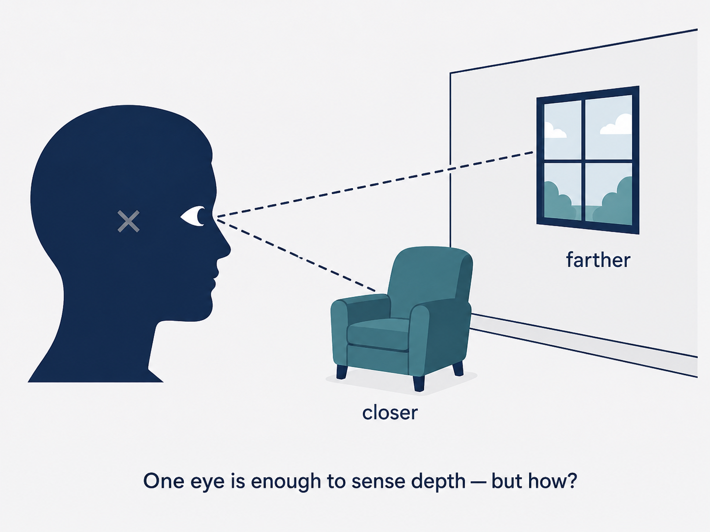
For decades, computer vision researchers assumed this was essentially impossible to automate reliably. Depth, they argued, is fundamentally lost when a 3D scene is projected onto a 2D sensor — the math is irreversible. And in a strict geometric sense, they were right. But as this article will show, geometry is not the only source of depth information. Texture gradients, occlusion patterns, lighting, shadows, and the statistical regularities of natural scenes all carry depth signals that a sufficiently powerful learning system can exploit.

This article explores two closely related problems that sit at the heart of modern computer vision: monocular depth estimation (recovering depth from a single image) and feature tracking (consistently identifying the same physical points across a sequence of images). Both problems, at their core, are instances of the same fundamental challenge — the correspondence problem — and modern deep learning has transformed how we attack both. We’ll trace the intellectual journey from geometric first principles through supervised learning to the elegant self-supervised approaches that have pushed the state of the art, and we’ll examine the loss functions, architectures, and training tricks that make it all work.

The Correspondence Problem: The Thread Connecting Everything

Before diving into depth estimation specifically, it’s worth understanding the underlying problem that unifies much of geometric computer vision. The correspondence problem asks: given two or more images of the same scene, which pixel in image A corresponds to which pixel in image B?

This seems simple at first — just find the same point in both images. But in practice it is extraordinarily difficult. Lighting changes between images. Objects may be partially occluded. Regions of uniform texture (a white wall, a clear sky) offer no distinguishing information. Repetitive patterns (a brick facade, a tiled floor) create ambiguous matches. And at the scale of a full image with millions of pixels, brute-force search is computationally intractable.

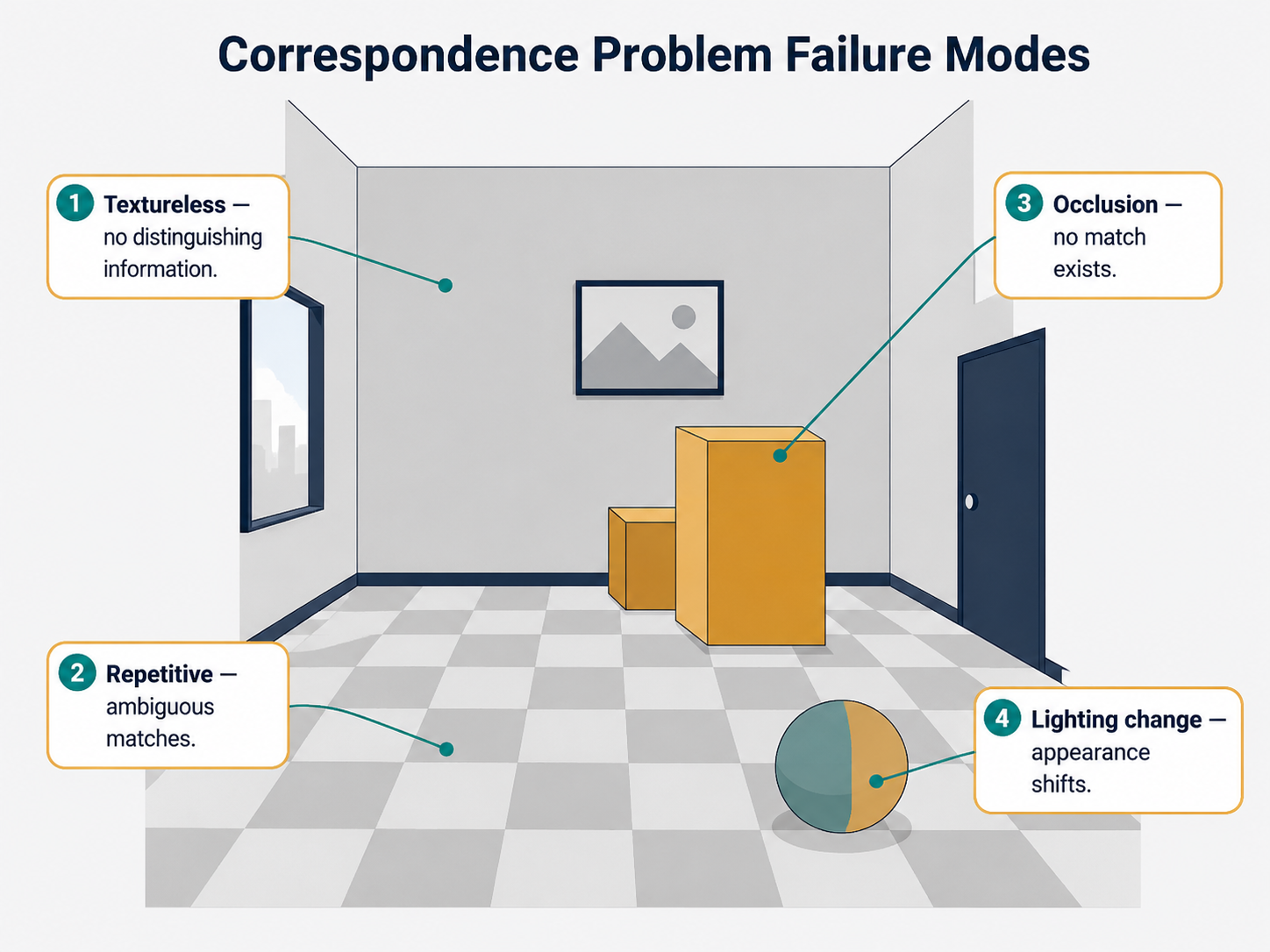
Both depth estimation and feature tracking are essentially specialized versions of solving this correspondence problem. For depth estimation, we want to find correspondences between a left camera image and a right camera image (or between frames in a video) so we can triangulate to recover 3D position. For feature tracking, we want to find correspondences for specific interesting points across many frames of video. The same techniques, the same mathematical tools, and — increasingly — the same deep learning architectures apply to both.

Part One: Monocular Depth Estimation

Why Depth Matters, and Why It’s Hard

Depth perception is a prerequisite for almost every meaningful interaction with the physical world. A robot arm reaching for an object needs to know how far away it is. An autonomous vehicle needs to know whether the pedestrian ahead is 5 meters away or 50. A 3D reconstruction pipeline needs per-pixel depth to build a model of a scene. Augmented reality systems need depth to occlude virtual objects correctly with real ones.

Active depth sensors like LiDAR (which fires laser pulses and measures return times) and structured light systems (which project known patterns and observe their deformation) solve this problem directly and accurately. But they are expensive, power-hungry, mechanically complex, and can struggle in bright outdoor environments where the ambient light washes out the sensor’s signal. A camera, by contrast, is cheap, passive, lightweight, and works anywhere.

The question is whether the information latent in a photograph is sufficient to recover depth — and, increasingly, the answer from deep learning is yes.

The Geometry of Stereo: Building Intuition for Depth from Disparity

To understand why depth estimation works at all, we need to first understand the stereo geometry that underlies it — even when we eventually move to a monocular (single-camera) setup.

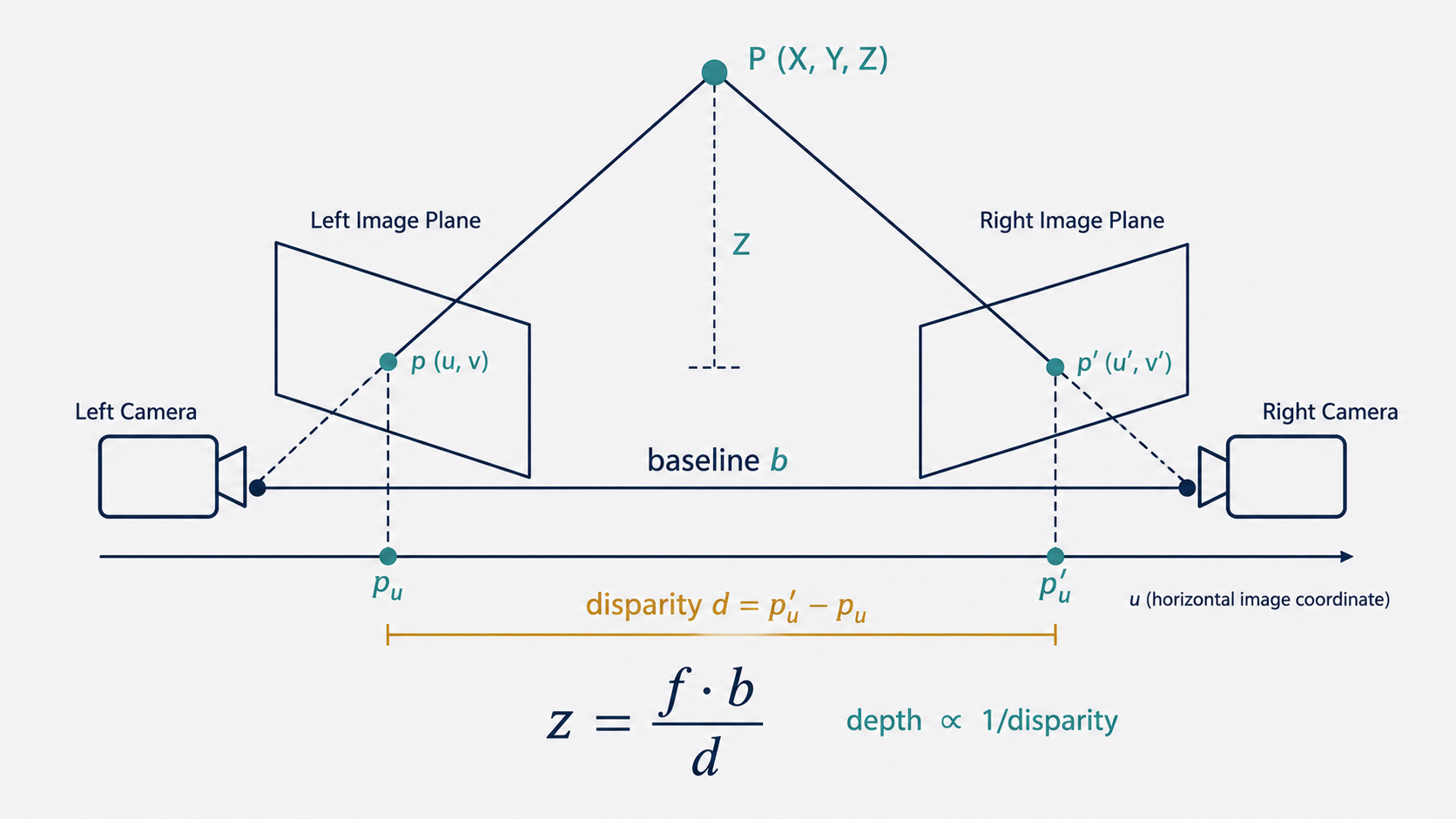
Imagine two cameras mounted side by side, their optical axes pointing in the same direction, separated by a horizontal distance $b$ called the baseline. This is exactly how your two eyes are arranged. When both cameras observe the same 3D point $P$, that point appears at slightly different horizontal positions in the two images. The farther away $P$ is, the smaller this horizontal shift. The closer it is, the larger the shift. This horizontal shift is called disparity, and it is the key to recovering depth.

To make this precise, consider the setup with the two camera image planes aligned (a configuration called rectified stereo). In this case, corresponding points in the two images lie on the same horizontal scan line — a constraint known as the epipolar constraint. The disparity $d$ between corresponding points $p$ (in the left image) and $p’$ (in the right image) is simply:

\[d = p'_u - p_u\]

where $p_u$ and $p’_u$ are the horizontal pixel coordinates in the left and right images respectively. By similar triangles relating the camera geometry, the depth $z$ of the point (its distance along the optical axis) is:

\[z = \frac{f \cdot b}{d} \tag{1}\]

Here, $f$ is the focal length of the cameras and $b$ is the baseline length. The relationship is elegantly simple and deeply intuitive: depth is inversely proportional to disparity. A point very far away produces nearly identical images in both cameras (small disparity, large depth). A point right in front of the cameras looks very different in the two views (large disparity, small depth).

This formula reveals something important: to recover depth, all we need to do is find correspondences between the two images. If we can identify which pixel in the right image corresponds to each pixel in the left image, we know the disparity everywhere, and therefore the depth everywhere. The depth estimation problem reduces to the correspondence problem.

A naive approach would search along each horizontal scan line in the right image for the best matching pixel, using raw pixel intensity or a small patch of pixels as the similarity metric. This works on simple, textured images but fails badly on textureless regions (uniform walls, clear skies), at depth discontinuities (object edges), and wherever occlusions exist (something visible in one camera is hidden in the other). Modern deep learning methods have largely superseded these naive matching approaches.

The Monocular Challenge: Geometry Becomes Ambiguous

Now consider the harder problem: estimating depth from a single image, with no stereo pair, no second viewpoint. Geometrically, this is fundamentally underconstrained. Any single image is consistent with infinitely many 3D scenes at infinitely many scales — a miniature model photographed close-up looks identical to a full-size building photographed from afar. There is no geometric operation you can perform on a single image that tells you absolute depth.

And yet humans manage it. When you look at a photograph, you immediately have a strong sense of the depth relationships in the scene. How? We exploit a rich set of learned visual priors: objects near the bottom of a scene tend to be closer than objects near the top (ground plane statistics); objects that appear smaller are typically farther away (size cues); texture gradients become finer with distance; familiar objects have known sizes (a car, a person); shadows and shading reveal surface orientation; partial occlusion tells us which surface is in front. None of these are geometric certainties — they are statistical regularities learned from a lifetime of experience with the 3D world.

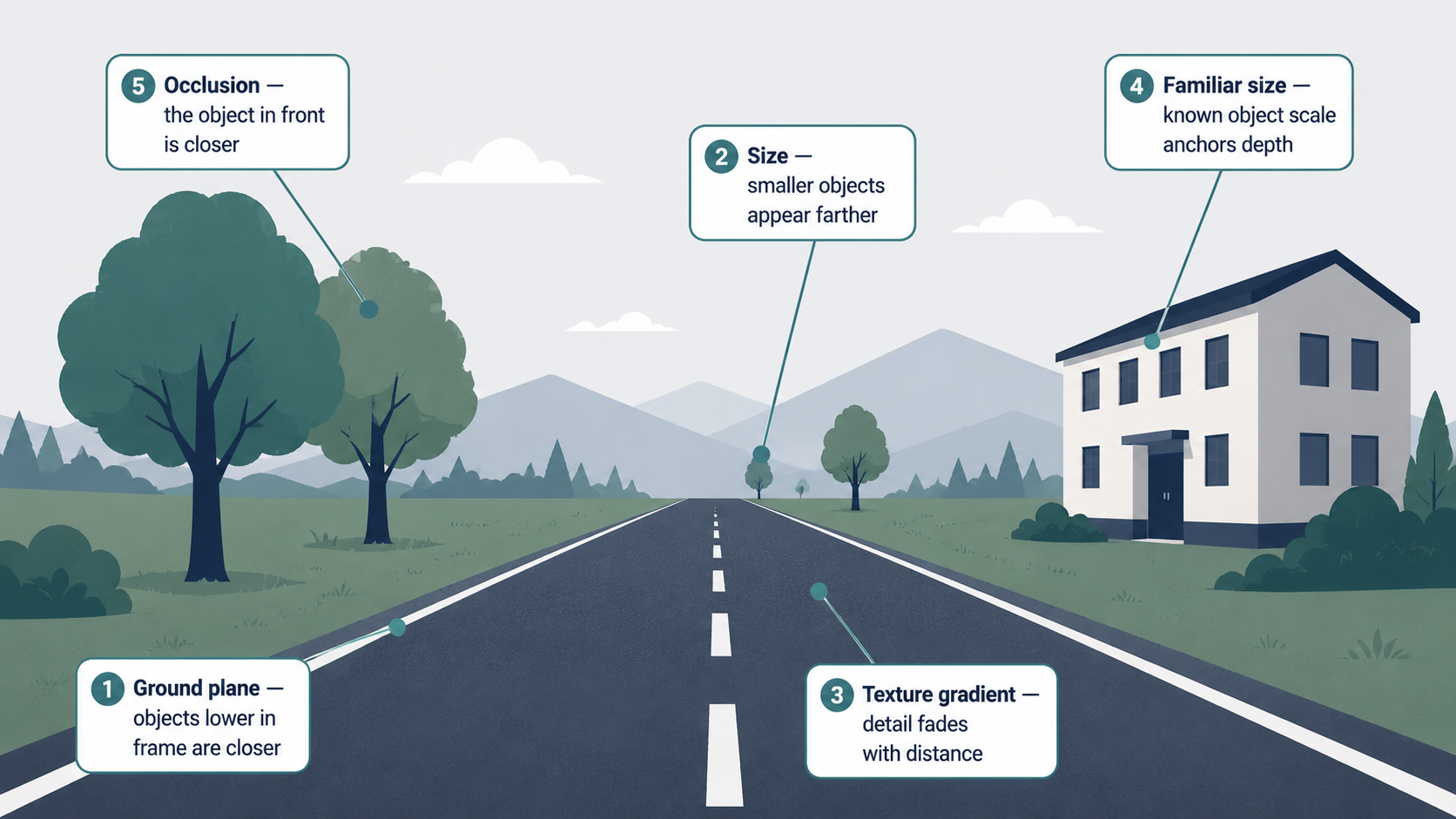
This is precisely the insight that motivates machine learning approaches to monocular depth estimation: if the regularities are statistical, a sufficiently powerful model trained on enough data should be able to learn them. The depth maps produced will be ambiguous in scale (we can’t know absolute distances without additional information), but relative depth relationships can be estimated well.

Supervised Depth Estimation: Learning with Ground Truth

The most conceptually straightforward approach is supervised learning. Collect a large dataset of RGB images paired with accurate depth maps (obtained from LiDAR sensors or other active methods). Train a convolutional neural network (CNN) to predict a depth or disparity map for each input image. The training loss measures the discrepancy between the network’s prediction and the ground truth depth, and gradient descent drives the network to minimize it.

This approach achieved impressive results and established that the problem was learnable. However, it has a critical practical limitation: ground truth depth data is expensive and difficult to collect at scale. LiDAR sensors are costly, their data is sparse (they don’t cover every pixel), and collecting large enough datasets across diverse scenes and conditions is a major logistical undertaking. The models trained on such data also tend to specialize to the domain they were trained in — a network trained on highway driving scenes may perform poorly in indoor environments.

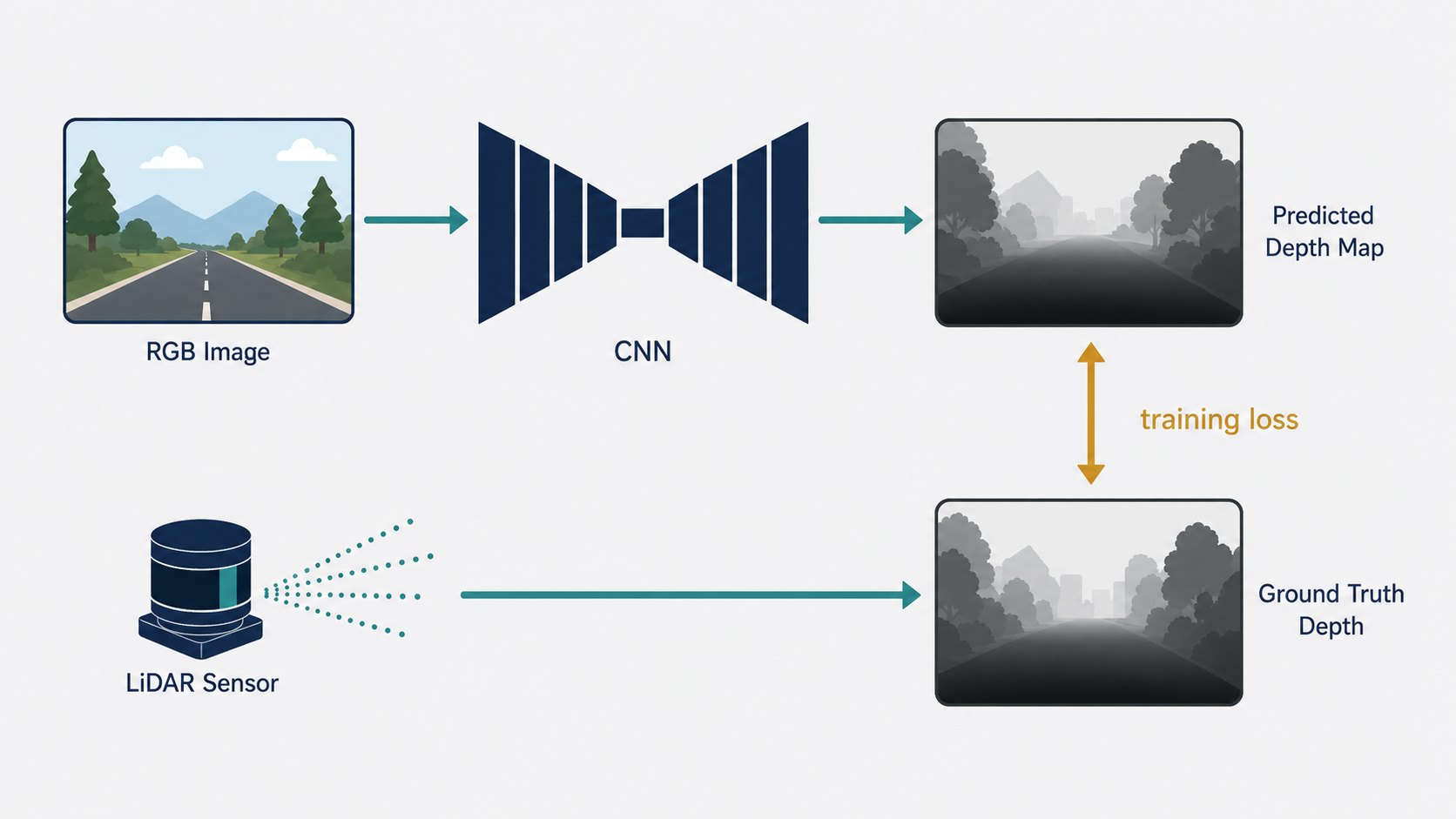
An important subtlety arises specifically in the monocular case: since there is no absolute scale information in a single image, networks can only recover depth up to scale. A network might consistently predict that near objects have depth values twice as large as far objects (correct relative depth) while being off by a constant factor on the absolute values. To handle this, researchers have proposed using scale-invariant error during training — a loss function that compares depth predictions in a way that is insensitive to the overall scale factor, focusing instead on getting the relative structure right.

Unsupervised Depth Estimation: Learning Without Labels

The limitations of supervised methods motivated a more elegant reformulation of the problem. Instead of requiring expensive ground truth depth annotations, could we train a depth estimation network using only raw stereo images — which are far cheaper to collect?

The key insight is a reframing: rather than predicting depth directly and comparing to ground truth depth, we can train the network to predict disparity as an intermediate representation for image reconstruction. If we can predict the disparity map for a left camera image, we can use that disparity map to synthesize (reconstruct) the left image by appropriately sampling from the right image. If our disparity predictions are accurate, the reconstructed left image should look like the real left image. This is the photometric reconstruction loss — a self-supervised signal that requires only paired stereo images, no depth labels at all.

Concretely, given a left image $I^l$ and right image $I^r$, a CNN processes the left image and outputs a disparity map $d^l$ — a per-pixel estimate of the horizontal shift needed to align corresponding pixels. The reconstruction is:

\[\tilde{I}^l(u, v) = I^r(u - d^l(u, v), v)\]

This says: to reconstruct pixel $(u,v)$ in the left image, look at the pixel in the right image that is $d^l(u,v)$ columns to the left. If the disparity is correct, the right image pixel at that location should have the same color as the left image pixel at $(u,v)$.

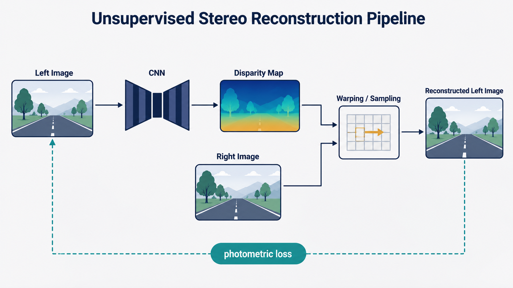
One subtlety: the disparity values $d^l(u,v)$ are continuous real numbers, but pixel coordinates must be integers. A pixel at the exact non-integer location doesn’t exist. The solution is bilinear interpolation — the reconstructed pixel value is computed as a weighted average of the four neighboring pixels in the source image, with weights determined by the fractional offset. Crucially, this interpolation is differentiable with respect to the disparity values, which means gradients can flow back through the sampling operation all the way to the CNN’s weights. This differentiable sampler is what makes end-to-end training possible.

A Rich Loss Function: Three Terms, Three Purposes

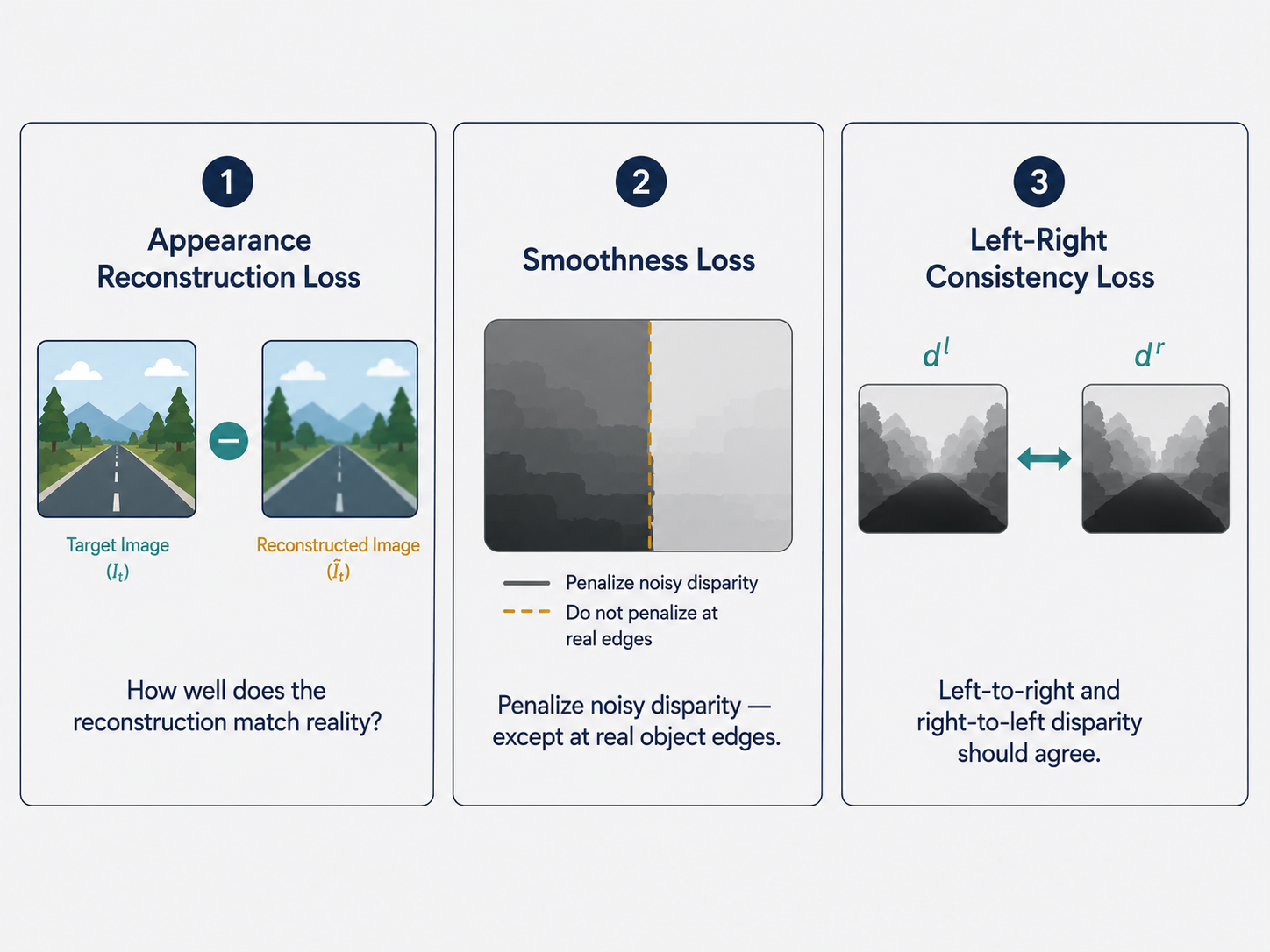
The most sophisticated version of this unsupervised approach predicts both a left-aligned and a right-aligned disparity map simultaneously, and reconstructs both images from each other. The total training loss at each spatial scale $s$ combines three distinct terms:

\[C_s = \alpha_{ap}(C^l_{ap} + C^r_{ap}) + \alpha_{ds}(C^l_{ds} + C^r_{ds}) + \alpha_{lr}(C^l_{lr} + C^r_{lr}) \tag{2}\]

Each term addresses a different aspect of what makes a good disparity map. Let’s unpack each one carefully.

The Appearance Reconstruction Loss ($C_{ap}$) is the core photometric signal. For each pixel $(i,j)$, it measures how well the reconstructed image matches the original:

\[C^l_{ap} = \frac{1}{N} \sum_{i,j} \alpha \frac{1 - \text{SSIM}(I^l_{ij}, \tilde{I}^l_{ij})}{2} + (1 - \alpha) \|I^l_{ij} - \tilde{I}^l_{ij}\| \tag{3}\]

This is a weighted combination of two similarity measures. The L1 term $|I^l_{ij} - \tilde{I}^l_{ij}|$ measures simple per-pixel intensity difference. The SSIM term (Structural Similarity Index) is more sophisticated: it compares patches centered on each pixel along three dimensions — luminance (average brightness), contrast (standard deviation of brightness), and structure (correlation of local patterns). SSIM captures the perceptual quality of the reconstruction better than raw pixel differences, which is why it is weighted more heavily in practice ($\alpha = 0.85$).

The Smoothness Loss ($C_{ds}$) regularizes the disparity map by penalizing rapid, unexplained changes in disparity:

\[C^l_{ds} = \frac{1}{N} \sum_{i,j} |\partial_x d^l_{ij}| e^{-\|\partial_x I^l_{ij}\|} + |\partial_y d^l_{ij}| e^{-\|\partial_y I^l_{ij}\|} \tag{4}\]

The intuition here is subtle and worth dwelling on. In general, depth maps should be smooth — nearby pixels on the same surface usually have similar depths, so abrupt changes in disparity should be penalized. However, at object boundaries, depth genuinely does change abruptly: the foreground object has one depth and the background has another, and there’s a sharp edge between them. We don’t want to penalize disparity gradients at these real edges.

The exponential weighting term is the solution. When the image gradient $|\partial_x I^l_{ij}|$ is large (we’re at a high-contrast edge in the image), the factor $e^{-|\partial_x I^l_{ij}|}$ becomes small, relaxing the smoothness penalty. When the image gradient is small (we’re in a textureless region), the exponential is close to 1, and the smoothness penalty is enforced strongly. This design elegantly couples disparity smoothness to image structure, allowing sharp disparity at image edges while suppressing noisy disparity in flat regions.

The Left-Right Consistency Loss ($C_{lr}$) enforces a geometric self-consistency between the two predicted disparity maps:

\[C^l_{lr} = \frac{1}{N} \sum_{i,j} |d^l_{ij} - d^r_{ij + d^l_{ij}}| \tag{5}\]

The logic is intuitive: the disparity of a pixel computed going from left-to-right should match the disparity computed going from right-to-left. If pixel $(i,j)$ in the left image has left-aligned disparity $d^l_{ij}$, then the corresponding pixel in the right image is at position $j + d^l_{ij}$. The right-aligned disparity at that position should equal $d^l_{ij}$. Any discrepancy signals an inconsistency in the predictions — perhaps caused by occlusion, where a region visible in the left camera is hidden in the right, making the disparity locally unreliable.

Together, these three loss terms — reconstruction quality, spatial smoothness, and geometric consistency — shape the network into producing disparity maps that are photometrically accurate, spatially regular, and geometrically coherent. The result, remarkably, is a monocular depth estimator trained entirely without ground truth depth labels.

Self-Supervised Depth Estimation: The Video Formulation

The unsupervised approach described above still requires synchronized stereo image pairs at training time. A subsequent generation of methods removed even this requirement, enabling training on ordinary monocular video — the most abundant and cheapest source of visual data imaginable. This is the domain of self-supervised depth estimation.

The reframing is elegant: instead of reconstructing the left image from the right image using predicted disparity, we frame depth estimation as a novel view synthesis problem. Given a video frame $I_t$ at time $t$, can we predict what the scene would look like from the camera’s position at time $t-1$ or $t+1$?

If depth estimation is correct and we know how the camera moved between frames, then we can take any pixel $(u,v)$ in frame $I_t$, use the predicted depth $D_t$ to backproject it to a 3D point in space, apply the camera’s relative pose transformation to find where that 3D point falls in the coordinate system of the adjacent frame, and project it forward to get pixel coordinates $(u’, v’)$ in the source frame $I_{t’}$. The synthesized view of $I_{t’}$ is simply: $\tilde{I}_{t’}(u’, v’) = I_t(u, v)$.

The pipeline requires two parallel networks:

The depth network takes a single color frame $I_t$ and outputs a dense depth map $D_t$, using a convolutional encoder-decoder architecture (the encoder compresses the image into a compact feature representation, the decoder expands it back to a full-resolution depth map).

The pose network takes a pair of adjacent frames $(I_t, I_{t’})$ and outputs the relative camera pose $T_{t \to t’}$ — the rotation and translation describing how the camera moved between the two frames.

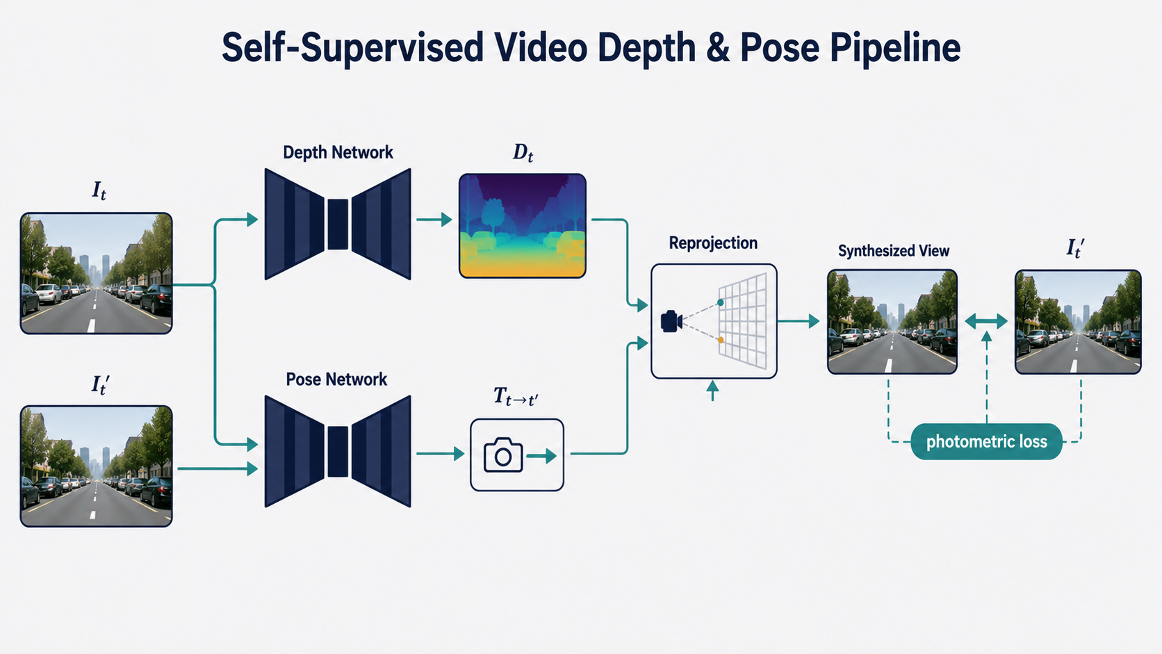
Given $D_t$, $T_{t \to t’}$, and the known camera intrinsics $K$, the reprojection pipeline synthesizes novel views, and the training signal is the photometric error between the synthesized view and the actual observed frame:

\[pe(I_a, I_b) = \frac{\alpha}{2}(1 - \text{SSIM}(I_a, I_b)) + (1 - \alpha)\|I_a - I_b\|_1 \tag{6}\]

The total photometric loss sums over both adjacent frames:

\[L_p = \sum_{t'} pe(I_t, I_{t' \to t}) \tag{7}\]

The depth map $D_t$ is optimized so that reprojecting pixels from the current frame into adjacent frames produces views that are as photometrically similar as possible to the actually observed frames. Errors in the depth prediction will cause reprojected points to land at the wrong locations in the adjacent frames, producing blurry or misaligned synthesized views and increasing the loss.

The self-supervised formulation is powerful because it requires nothing more than unlabeled video. Any dashcam footage, any handheld video, any robot traversing an environment — all of this becomes training data. This abundance of data, combined with the photometric supervision signal inherent in temporal coherence, allows self-supervised methods to match and in some cases exceed the performance of supervised approaches trained on expensive labeled datasets.

Part Two: Feature Tracking

The Problem: Following Points Through Time

Imagine watching a video of a person walking across a room. If you fix your attention on a button on their jacket, you can follow that button through every frame — even as the person turns, the lighting shifts, and the button’s appearance changes. You’re solving the feature tracking problem: maintaining consistent identity for a set of image points across a temporal sequence.

Formally, feature tracking means: given a sequence of images and an initial set of 2D points in the first frame, find the corresponding locations of those same points in all subsequent frames. Like depth estimation, this is another instantiation of the correspondence problem — but now the correspondences span time rather than space.

Feature tracking is a building block for a wide range of applications. Visual odometry and SLAM (Simultaneous Localization and Mapping) systems track features to estimate camera motion. Object tracking systems follow distinctive points on objects of interest. Video stabilization corrects for camera shake by measuring feature motion. Motion capture systems track markers on performers’ bodies. In each case, the reliability of downstream results depends entirely on the quality of the feature tracks.

What Makes a “Good” Feature?

Not every pixel in an image is equally trackable. A pixel sitting in the middle of a uniformly colored wall is essentially impossible to track reliably — if it moves slightly, it looks identical to its neighbors, and there’s no way to tell which pixel in the next frame corresponds to it. This is the aperture problem: when you can only see a small patch of a uniform region, you can’t tell whether it has moved horizontally, vertically, or diagonally.

What we want are image regions that are distinctive in multiple directions simultaneously — regions where the local appearance is unique enough that displacement in any direction produces a noticeably different patch. Corners are the archetypal example: a corner has strong gradients in two orthogonal directions, making it uniquely identifiable. An edge only has a strong gradient perpendicular to the edge, so it can only be localized in one direction. A flat region has no strong gradients and cannot be localized at all.

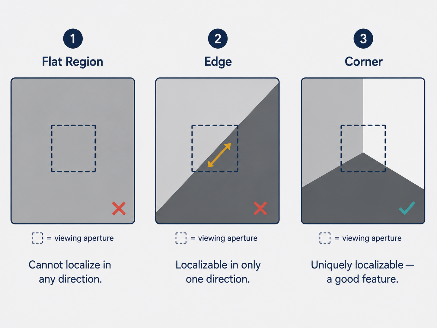
This intuition motivated decades of research into hand-designed feature detectors: methods like Harris corners, SIFT (Scale-Invariant Feature Transform), SURF, and ORB all attempt to find image locations that are distinctive, repeatable under viewpoint changes, and efficiently describable. These methods also produce descriptors — compact numerical summaries of the local image patch around each detected feature point, designed to be similar for the same physical point seen from different viewpoints and different from unrelated points.

Traditional descriptor-based methods are sparse — they only compute descriptors for a small fraction of pixels in the image (the “interesting” ones). They are also hand-engineered — a domain expert decided what mathematical properties make a good descriptor. Both of these limitations motivated the move to learned descriptors.

Learned Dense Descriptors: Teaching the Network What “Same” Means

Instead of hand-crafting the rules for what makes a good feature descriptor, we can learn them from data. The approach is conceptually clean: train a neural network to assign each pixel in an image a high-dimensional descriptor vector, such that pixels corresponding to the same 3D point (across different images) get similar descriptor vectors, while pixels corresponding to different 3D points get different descriptor vectors.

The network $f(\cdot)$ maps an input image $\mathbb{R}^{W \times H \times 3}$ to a descriptor image $\mathbb{R}^{W \times H \times D}$ — every pixel gets a $D$-dimensional descriptor. This is dense: every pixel is described, not just a sparse set. The convolutional encoder-decoder architecture is again appropriate here, as it naturally produces outputs at the same spatial resolution as the input.

To visualize what the network has learned, we can project the $D$-dimensional descriptors down to 3 dimensions using PCA or t-SNE and display the result as an RGB image. Regions of the object that are semantically or structurally similar will appear as similar colors, revealing the structure the network has discovered in the descriptor space.

The training objective is a pixel-contrastive loss that operates on pairs of images $(I_a, I_b)$ of the same scene or object from different viewpoints, along with a list of known ground-truth correspondences between them. The loss has two complementary components:

The match loss pulls corresponding descriptors together:

\[L_{\text{matches}}(I_a, I_b) = \frac{1}{N_{\text{matches}}} \sum_{N_{\text{matches}}} D(I_a, u_a, I_b, u_b)^2 \tag{8}\]

For each known ground-truth match $(u_a, u_b)$ — a pair of pixel locations in $I_a$ and $I_b$ that image the same 3D point — we compute the squared L2 distance between their descriptors and minimize it. The network learns to map corresponding pixels to nearby points in descriptor space.

The non-match loss pushes non-corresponding descriptors apart:

\[L_{\text{non-matches}}(I_a, I_b) = \frac{1}{N_{\text{non-matches}}} \sum_{N_{\text{non-matches}}} \max(0, M - D(I_a, u_a, I_b, u_b)^2) \tag{9}\]

For each known non-match $(u_a, u_b)$ — a pair of pixel locations that do NOT correspond — we want the descriptor distance to be large (at least $M$, the margin). If the distance is already greater than $M$, the loss is zero (the pair is already sufficiently separated). If the distance is less than $M$, we penalize proportionally to how much the descriptors are overlapping in descriptor space. This is the hinge loss structure, standard in contrastive learning.

The total loss combines both:

\[L(I_a, I_b) = L_{\text{matches}}(I_a, I_b) + L_{\text{non-matches}}(I_a, I_b) \tag{10}\]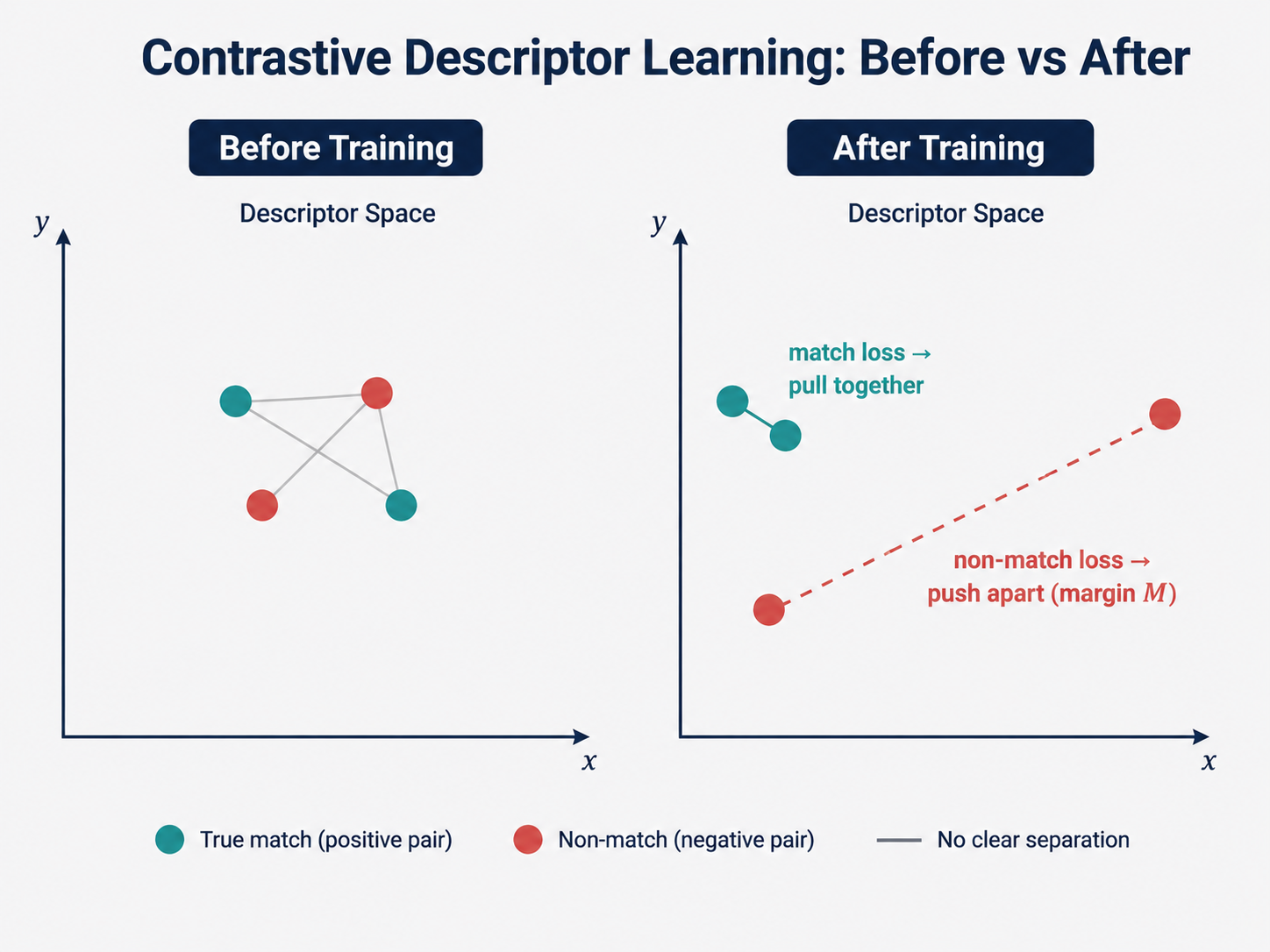

The intuition is beautiful: the network is essentially being told “points that see the same thing should be close together in descriptor space; points that see different things should be far apart.” Given enough examples of what “same” and “different” look like, the network learns to embed visual content into a space where proximity means correspondence.

The Data Problem: Getting Correspondences Without Labels

The contrastive loss requires ground-truth correspondences — we need to know which pixels in image $I_a$ match which pixels in image $I_b$. How do we get these at scale without enormous human labeling effort?

The elegant solution uses a robotic arm. Mount a camera on the end of a robotic arm. Place an object on a table. Command the arm to move to many different positions around the object, taking a photograph at each position. Since the forward kinematics of the arm are precisely known, we know the exact 6-DOF pose of the camera at every position. Using these poses and all the images, we can run a standard multi-view 3D reconstruction algorithm (structure-from-motion) to build a 3D model of the object. Given the 3D model and the camera poses, we can automatically generate as many ground-truth pixel correspondences as we want — project any 3D point into any pair of camera views and record the pixel locations. The robot generates its own labeled training data, fully autonomously.

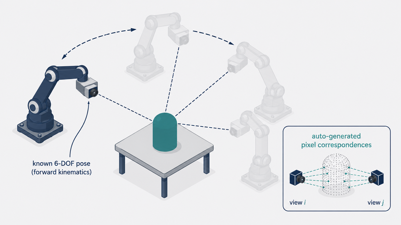
This self-supervised data collection strategy is powerful because it produces dense, precise correspondence labels at essentially zero human cost. Additional tricks further improve the learned descriptors: background randomization (randomly replacing the background in training images) prevents the network from using background context to identify object parts; data augmentation (random crops, color jitter, flips) improves robustness; and hard-negative mining (preferentially sampling non-matches that are visually similar and thus most likely to confuse the network) trains the network to discriminate at the margins where discrimination matters most.

Cross-Object Generalization and Class-Consistent Descriptors

An interesting challenge arises when the network is trained only on images of individual objects: the learned descriptors may lack the ability to distinguish between different objects, because the training never required it. A network trained only on a single caterpillar toy might assign similar descriptors to corresponding parts of two completely different toys.

The fix is straightforward: add a cross-object loss, treating all pixel pairs from images of two different objects as non-matches. This forces the network to separate descriptor clusters for different objects. The result, visualized in descriptor space via dimensionality reduction, shows distinct clusters for distinct objects — the network has learned that different objects should occupy different regions of descriptor space.

Perhaps even more interesting is class-consistent correspondence: when the network is trained on multiple objects of the same class (say, multiple different baseball caps), it learns to assign semantically consistent descriptors to functionally corresponding parts, even across objects with different visual appearances. The brim of one cap maps to the same region of descriptor space as the brim of another cap, even if the caps are different colors and designs. The network has learned a functional concept — “brim-ness” — purely from the geometric consistency of how brims appear across different viewpoints and instances.

The Common Thread: Representation Learning as the Foundation

Looking back across both problems — depth estimation and feature tracking — a unifying theme emerges. In both cases, the most successful modern approaches frame the problem as representation learning: we want to learn an intermediate representation (a depth map, a disparity map, a descriptor vector) that captures something meaningful about the 3D structure of the world.

In depth estimation, the representation is the depth or disparity map, and the learning signal comes from photometric consistency — the requirement that predicted depths, when used to reproject pixels between views, should produce images that look like real images.

In feature tracking, the representation is the descriptor field, and the learning signal comes from contrastive correspondence — the requirement that pixels imaging the same 3D point should have nearby descriptors, while pixels imaging different points should have distant descriptors.

In both cases, the crucial insight is that we can obtain useful training signals without explicit human labels, by exploiting the rich geometric and photometric structure that already exists in multi-view image data. The 3D world imposes strong constraints on how images relate to each other — constraints that a learning system can leverage as self-supervision.

Practical Implications and Applications

The techniques discussed here have moved far beyond academic interest into deployment at scale.

Autonomous driving systems from companies ranging from Tesla to Waymo use variants of these ideas. Monocular depth estimation supplements or provides a fallback for expensive LiDAR sensors. Feature tracking forms the backbone of visual odometry, allowing vehicles to estimate their own motion through an environment by watching how image features move across video frames.

Robotics uses dense descriptor learning (in the form of systems like Dense Object Nets) for manipulation tasks. A robot can be trained to grasp the same point on an object across different poses and appearances, because the learned descriptor at that point is consistent regardless of viewpoint. This enables robust, appearance-independent grasping without requiring explicit 3D object models.

Augmented and mixed reality systems use feature tracking extensively to maintain stable alignment of virtual content with the real world. The accuracy and robustness of the feature tracker directly determines whether virtual objects appear solidly anchored in space or jitter and drift.

Video understanding — action recognition, activity detection, video search — uses feature tracking and learned representations to capture the dynamics of scenes over time, going beyond the static analysis of individual frames.

Conclusion: Geometry, Supervision, and the Power of Self-Consistency

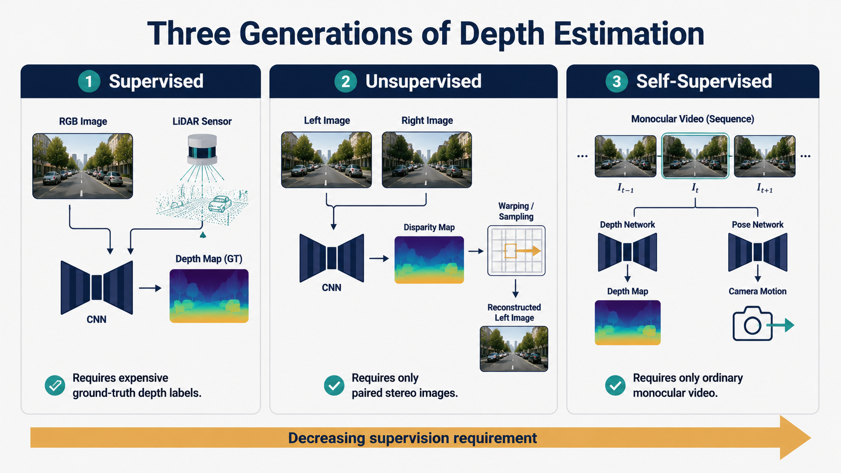
We have traveled from the clean geometry of stereo triangulation — depth is inversely proportional to disparity, recoverable if you can find correspondences — through the challenge of monocular depth estimation (geometrically underconstrained, but statistically learnable), and across three generations of learning paradigms:

Supervised methods use explicit depth ground truth as the training signal, achieving good performance but requiring expensive labeled data. The scale ambiguity inherent in monocular depth is handled through scale-invariant loss functions.

Unsupervised methods bypass the need for depth labels by formulating the problem as stereo image reconstruction. The photometric loss, differentiable sampling, smoothness regularization, and left-right consistency together shape a rich training signal purely from stereo image pairs.

Self-supervised methods remove even the stereo requirement, training on monocular video by formulating depth estimation as novel view synthesis. A depth network and a pose network are jointly trained through photometric consistency across time.

For feature tracking, learned dense descriptors replace hand-engineered features with networks trained via contrastive correspondence losses, producing dense, viewpoint-invariant representations with class-consistent semantics.

The central lesson woven through all of these approaches is that the 3D world is structured and consistent in ways that images faithfully record. Photometric consistency, geometric coherence, temporal continuity — these are not just properties of the world but sources of supervision that a learning system can exploit. We don’t always need humans to tell the system what depth is or what features are; we can let the geometry of the world do the teaching.

That is, perhaps, the deepest insight in this entire field: the labels we need to teach machines about 3D vision have been embedded in every pair of photographs, every second of video, every stereo image ever taken. We simply needed to learn how to read them.

This article is based on CS231A Course Notes 8: Monocular Depth Estimation and Feature Tracking, by Kenji Hata and Silvio Savarese, Stanford University.

Monocular Depth Estimation and Feature Tracking